Simulation runs a model under stated assumptions. A two-state stock example shows why physical-world cash-flow forecasts and risk-neutral option prices differ.
Simulation
Simulation is the execution of a model to reproduce how a system behaves under specified inputs and assumptions. A quant might simulate a portfolio through future market scenarios, replay a trading rule with transaction costs, or generate the cash flows of an option. The output describes what the model does; it is not an observation of what the market will do.
Simulation can be deterministic, with fixed inputs, or stochastic, with random inputs. Monte Carlo simulation repeatedly samples those random inputs to estimate quantities such as prices, expected losses and breach probabilities. Stochastic modelling specifies the uncertain mechanism; simulation runs it; a Monte Carlo estimator turns the outputs into an estimate.
Decide which question the model answers
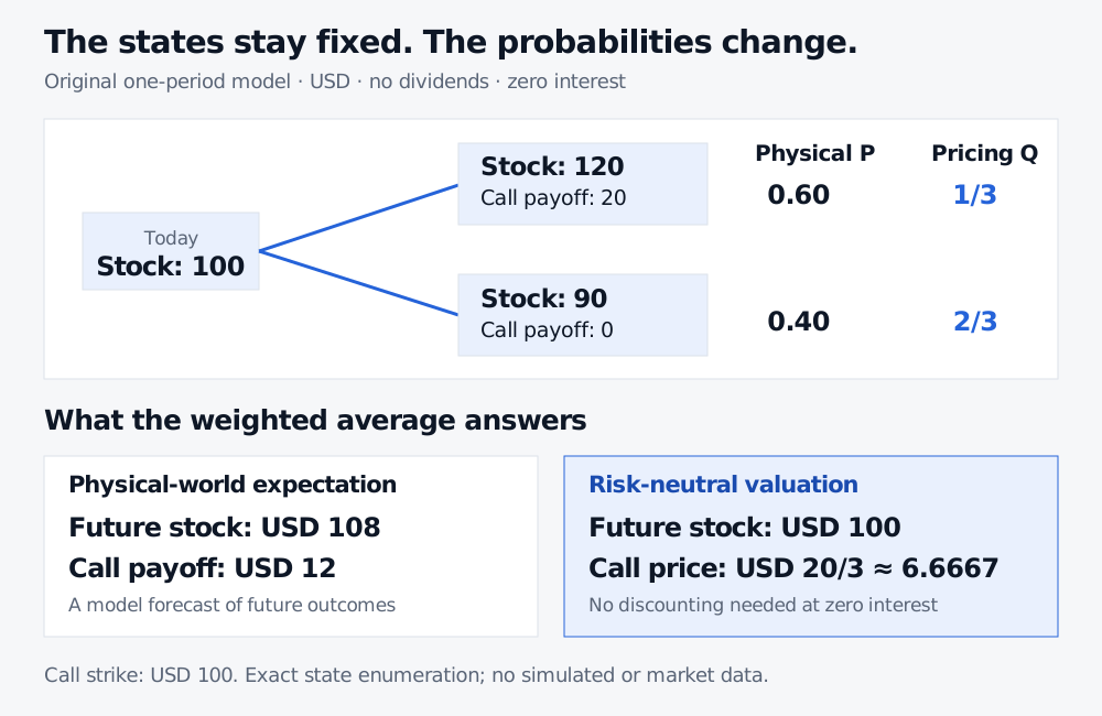
Suppose a non-dividend-paying stock costs USD 100 today. Over one period it ends at USD 120 with physical probability 0.60, or USD 90 with probability 0.40. A European call with strike USD 100 therefore pays USD 20 or USD 0.
To illustrate the arithmetic, construct 100 one-period paths: 60 up and 40 down. The average terminal stock value is USD 108 and the average call payoff is USD 12. These counts are stipulated, not the result of a random simulation. In an actual run of 100 independent draws, the up count fluctuates; it need not equal 60.
Does USD 12 price the call? Under this frictionless, complete two-state model, with unrestricted stock and cash trading and a zero interest rate, the answer is no. Pricing uses the risk-neutral measure, whose up probability makes the stock's expected terminal value equal its current value:
q(120)+(1−q)(90)=100⟹q=31.
At zero interest, the risk-neutral expected payoff is already its present value:
C0=31(20)+32(0)=320 USD≈6.6667 USD.
A stock moves from USD 100 to USD 120 or USD 90. Physical probabilities 0.60 and 0.40 give an expected stock value of USD 108 and call payoff of USD 12. Risk-neutral probabilities one third and two thirds give an expected stock value of USD 100 and zero-rate call price of USD 20/3.
Original one-period model, not market data. Both calculations use the same stock states and call payoffs; the probability weights determine which question is answered.
An independent replication check holds 2/3 of a share and borrows USD 60. Its terminal value is USD 20 in the up state and USD 0 in the down state. Its initial cost is (2/3)(100)−60=20/3 USD, matching the price above. The physical up probability does not enter this hedge calculation. The freely accessible Binomial Model sample lesson develops this link between replication and risk-neutral valuation.
This two-state problem needs only exact enumeration. Simulation becomes useful when the model has too many paths or interacting features to enumerate conveniently. Running more physical-world paths would refine an estimate of USD 12; it would not convert that expectation into the model's no-arbitrage price.
What to specify before running
A useful simulation description identifies the model and its inputs, the horizon and observation dates, the probability law or fixed scenarios, and the output being measured. “One million paths” says little without those choices. A terminal stock value, a path minimum and a discounted call payoff are different outputs from the same underlying model.
For stochastic runs, record the generator, its version and the random seed, together with the other inputs. Reproducing a run helps detect changes and compare methods; it does not establish that the model is appropriate. For seeded code that develops the sample-average calculation, see Simulation and Resampling, a membership lesson with a public preview.
Keep three questions separate when interpreting the result:
Sampling precision: how much would a stochastic estimate vary across independent runs? More draws can reduce this uncertainty under the estimator's assumptions.
Numerical approximation: does the implementation approximate the intended model or payoff accurately? A coarse time discretisation can miss events between observation dates; adding paths on the same grid does not repair that bias.
Model relevance: do the assumptions and inputs suit the intended decision? More computation does not remove model risk.
A simulated loss distribution is useful because it makes the consequences of assumptions calculable. Interpreting it still requires knowing which assumptions produced it.
Sources
Paul Glasserman, Monte Carlo Methods in Financial Engineering (2003), §§1.1.1–1.1.3 and §1.2.1: simulation estimators, discretisation bias and pricing by replication. Springer.
Mike Giles, Monte Carlo Methods, Lecture 1, slides 1–8: financial simulation, model paths and discounted-payoff averaging. University of Oxford lecture notes.