Stochastic modelling is the construction and use of mathematical models that assign probabilities to uncertain outcomes or histories. In finance, it turns a question such as “how many orders might fill?” into a distribution that can inform an execution decision. The randomness belongs to the model: whether its probabilities describe the market well is a separate question requiring evidence.
A model needs more than a distribution name. It needs a question, a state that records what matters, a time scale, a probability law, data for choosing its inputs, and checks tied to its intended use. A stochastic process is one mathematical ingredient when the state evolves through time; stochastic modelling also includes deciding what to leave out and whether that simplification is tolerable.
A small execution model
Suppose a desk wants the distribution of filled orders among its next ten submissions. For this synthetic example, each order uses the same execution rule and the same observation window. Define a fill as complete execution within that window; partial execution counts as zero. Let be one for a fill and zero otherwise. Time is indexed by order number, rather than clock time.
Assume the future indicators are mutually independent and follow the same Bernoulli distribution, with unknown fill probability . Those are substantive modelling choices. A common order rule does not establish independence or a constant probability: queue position, spread and volatility could change both.
Five earlier, comparable orders produced
Under the stipulated independent Bernoulli model, the sample proportion is the maximum-likelihood estimate of . Five observations are used here to make the arithmetic visible, not to recommend an adequate dataset for an execution system.
Now plug in and hold it fixed. The future count has the model distribution
The subscript marks a forecast evaluated at the fitted parameter. The binomial distribution gives
The mean is six filled orders; the variance is 2.4 orders squared. Zero fills has model probability about 0.0105%. Six is an average over hypothetical repetitions, not a promise about the next batch.
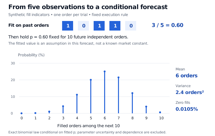
Original synthetic example. Exact probabilities for ten independent future orders with the fitted probability held fixed; estimation uncertainty and dependence are excluded.
This distribution describes outcome uncertainty conditional on a chosen parameter, not the full uncertainty of the forecasting exercise. The true is unknown. Incorporating parameter uncertainty requires an additional inferential treatment; the plug-in calculation does not supply one automatically. Dependence is another omission: if fills cluster with liquidity conditions, the count law need not be binomial even when the average fill probability remains 0.60.
Fitting is not checking
Estimating from past fills is calibration. Reproducing the same sample's fill rate is built into that fit; it provides little evidence that the next ten orders follow the assumed law.
Useful validation would compare forecasts with later, unused orders, examine whether errors cluster by market condition, and assess whether the fill definition and recorded data match the desk's actual decision. Testing alternative probabilities and dependence assumptions asks how sensitive that decision is to plausible model changes. The Federal Reserve's model-risk guidance, sections IV–V, distinguishes development and testing from validation, including conceptual soundness, outcomes analysis and ongoing monitoring. A correct calculation can still support a poor decision when its assumptions or use are unsuitable.
Simulation is optional here: the exact count law is available. Monte Carlo simulation becomes useful for richer execution histories, but generating more paths reduces simulation noise, not parameter uncertainty or model misspecification.
Choose probabilities for the question
The fill forecast aims to describe actual outcomes, a physical-measure or question. Derivative valuation commonly uses a risk-neutral measure, , whose probabilities serve no-arbitrage pricing rather than forecasts of observed frequencies. Switching between them changes the question being answered.
For a financial application of this distinction, §2.1 of Stochastic Modelling for Retirement Products separates retirement scenario planning from guarantee valuation. The public page is a preview; the full lesson requires membership. Before choosing a sophisticated process, decide which of those tasks the model must perform.
Sources
- John A. Rice, Mathematical Statistics and Data Analysis, 3rd ed. (2007), §§2.1.1–2.1.2: Bernoulli indicators and counts of independent trials.
- NIST/SEMATECH, “Binomial Distribution”: probability mass function, moments and maximum-likelihood estimator.
- Federal Reserve, “Supervisory Guidance on Model Risk Management”, sections IV–V: model development, validation and monitoring.