Discretisation: Definition & Examples

Discretisation replaces a continuous description with values, equations or decisions on a discrete set. A numerical option pricer may replace continuous time by dates, an underlying-price interval by grid nodes, and derivatives by differences between nearby values. The resulting calculation solves an approximation whose behaviour depends on those choices.

That matters even when the financial model is unchanged. Moving from monthly to daily simulation can alter a price because the approximation changes. Changing a contract from continuous to monthly barrier monitoring instead changes the payoff being priced. Both involve discrete dates, but they answer different questions.

Three choices hidden inside “use a grid”

Choice	What becomes discrete?	What still needs specifying?
Time grid	Dates $t_n=nh$ replace all times in an interval.	Step size $h$ , terminal date, and a rule for advancing the state.
State grid	Selected underlying prices or other state coordinates replace a continuum of locations.	Spacing, domain limits, boundary conditions and interpolation.
Equation approximation	A derivative or integral is replaced by a finite formula.	Which neighbouring values enter, where coefficients are evaluated, and the approximation's error.

These choices can be made separately. A time-stepped simulation may keep the state continuous: a simulated asset value need not be rounded to a price lattice. Conversely, discretising space in a partial differential equation can leave a system of continuous-time equations to solve. Finite-difference methods commonly combine space, time and derivative approximations.

A continuous decay becomes a recurrence

Take a deliberately simple ordinary differential equation:

\frac{dy}{dt}=-\kappa y,\qquad y(0)=1, \qquad \kappa=1\text{ per year}.

The state $y$ is dimensionless and time is measured in years. This could represent a synthetic remaining-exposure fraction under a constant proportional run-off assumption. It is an illustrative model, not an estimated exposure forecast. Its exact solution is $y(t)=e^{-\kappa t}$ , so at one year the target is $e^{-1}\approx0.367879$ .

Choose $N$ equal time steps over $T=1$ year, with $h=T/N$ . The forward Euler method replaces the time derivative by a forward difference and evaluates the slope at the old state:

\frac{y_{n+1}-y_n}{h}=-\kappa y_n \quad\Longrightarrow\quad y_{n+1}=(1-\kappa h)y_n.

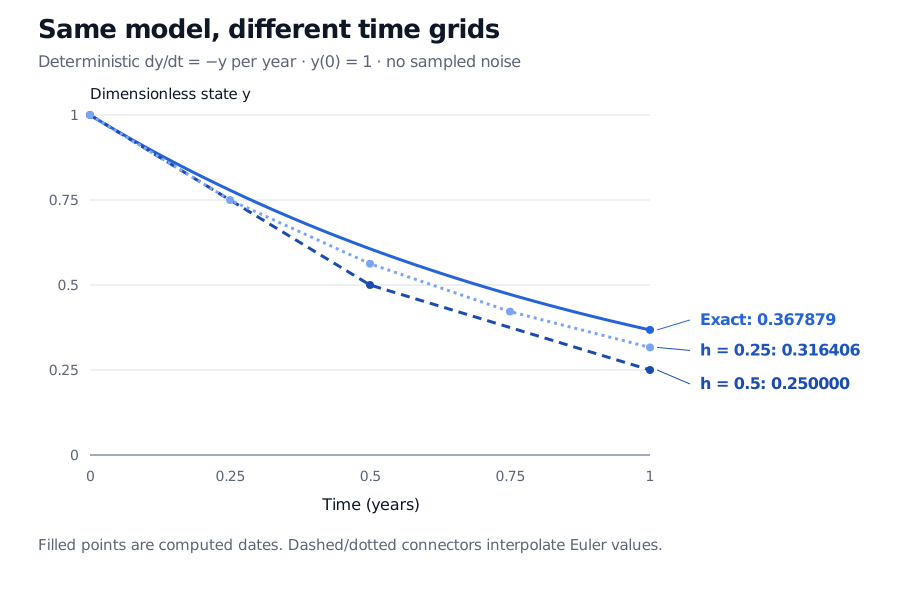
Here $y_n$ is a numerical approximation to $y(t_n)$ ; it is not a new exact solution of the continuous equation. The product $\kappa h$ is dimensionless. With half-year steps, the values are $1,1/2,1/4$ . With quarter-year steps, they are $1,3/4,9/16,27/64,81/256$ . Thus the one-year estimates are $0.25$ and $0.31640625$ , respectively.

Exact decay ends at 0.367879 after one year, compared with forward Euler values 0.25 with half-year steps and 0.316406 with quarter-year steps. All three start at 1.

Original deterministic calculation for proportional decay at 1 per year. Filled points are computed dates; dashed and dotted lines interpolate Euler values between them. The solid curve is the exact solution.

The discrepancy is discretisation error, even if every Euler operation is carried out with exact fractions. It is separate from rounding error. Sampling the exact solution at fewer dates would still give the correct values at those dates; Euler adds an approximation to the evolution between them. Driscoll and Braun's Euler derivation makes this distinction through the discrete recurrence and its error.

Refinement needs a target and an error measure

For this example, compare the computed and exact states at the same terminal date. The absolute endpoint error is

E_N=\left|(1-1/N)^N-e^{-1}\right|.

Steps $N$	Step $h$ (years)	Euler at one year	Absolute error
2	$1/2$	0.250000	0.117879
4	$1/4$	0.316406	0.051473
8	$1/8$	0.343609	0.024271
16	$1/16$	0.356074	0.011805

Values and errors are rounded to six decimal places. Halving the first step cuts the error by about

2.29

, rather than exactly two. The asymptotic claim is that this smooth problem has first-order global accuracy:

E_N

is proportional to

h

to leading order as

h\to0

with

T

fixed. It is not a promise of an exact factor-two improvement on every coarse grid. Convergence specifies the limiting process; order of accuracy describes its rate.

Damping and positivity are different tests

For the same decay equation and a fixed step $h>0$ , Euler repeatedly multiplies by $m=1-\kappa h$ . The exact positive solution decays to zero. Whether its numerical counterpart does so depends on the step:

Property of Euler on this scalar decay model	Condition
Magnitudes decay to zero as the number of steps grows	$\lvert1-\kappa h\rvert<1$ , or $0<\kappa h<2$
Every nonnegative starting state remains nonnegative	$1-\kappa h\ge0$ , or $\kappa h\le1$
Every strictly positive starting state stays strictly positive	$1-\kappa h>0$ , or $\kappa h<1$

For example,

\kappa h=1.5

gives multiplier

-0.5

: the sequence alternates signs while its magnitude decays. At

\kappa h=2

, multiplier

-1

is bounded but does not damp. Above 2, magnitudes grow. At

\kappa h=1

, Euler reaches zero immediately although the exact solution stays strictly positive. These distinctions explain why a numerically stable calculation may still violate a financial state constraint. Strang's MIT treatment develops this scalar stability test.

These thresholds belong to forward Euler on this particular decay equation. Other equations and schemes require their own analysis. For a positive growth rate, an increasing multiplier can reflect the growing exact model; it does not by itself diagnose numerical instability. Stability also does not certify small pricing error.

In practice, refine the dimensions that can affect the reported output: time, state spacing, truncated boundaries and payoff monitoring where relevant. Compare prices or sensitivities in their own units, keeping model and contract conventions fixed. Exact transitions for geometric Brownian motion remove its transition approximation at chosen dates, but cannot reveal a barrier crossing between them. More simulated paths reduce sampling noise; they do not automatically remove a fixed time-grid bias.

For the derivative-approximation part of this story, SelfMadeQuant's Numerical Differentiation derives forward and central differences and connects spacing to bumped Greeks. Its introduction and outline are public; the full lesson requires membership.

Sources

Stewart, J. Single Variable Calculus: Early Transcendentals, 6th ed., Thomson Brooks/Cole, 2008, §9.2, pp. 575–577: Euler steps and refinement.
Driscoll, T. A., and Braun, R. J., Fundamentals of Numerical Computation, §6.2, “Euler's method.”
Strang, G., MIT 18.086, 2006, Chapter 5, §5.1, “Finite Difference Methods”: forward Euler, scalar stability and fixed-horizon error.

Three choices hidden inside “use a grid”

A continuous decay becomes a recurrence

Refinement needs a target and an error measure

Damping and positivity are different tests

Sources

Related terms

Convergence of a numerical method

Geometric Brownian motion

Numerical stability

Order of accuracy

Rounding error