A Monte Carlo estimator turns simulated outputs into an estimate. See a USD 100 payoff example, unbiasedness, standard error and the limits of more draws.
Monte Carlo estimator
A Monte Carlo estimator is a statistic calculated from random simulations to approximate a target quantity. The basic version averages simulated outputs to estimate an expected value. In finance, each output might be a discounted derivative payoff, a portfolio loss or an indicator that a risk threshold was breached.
The estimator is the rule that turns scenarios into a number. Monte Carlo simulation supplies the scenarios; the estimator specifies what to compute from them. Before running either, state the target distribution and quantity. Averaging physical-world losses and averaging risk-neutral discounted payoffs answer different questions.
From one payoff to an average
Write the target as θ=E[Y]. Generate N independent, identically distributed outputs Y1,…,YN with the same law as Y. The plain sample-average estimator is
θ^N=N1i=1∑NYi.
Before drawing the sample, θ^N is a random variable. After drawing it, the calculated number is an estimate. When E[∣Y∣]<∞, this estimator is unbiased: its expectation equals θ. The law of large numbers also makes it converge to θ as the sample size grows. Neither statement promises that a particular finite run is correct.
For option valuation with a constant continuously compounded risk-free rate r, maturity T and payoff H, the usual risk-neutral representation gives Y=e−rTH and θ=EQ[Y]. Calculate the spread of these discounted outputs when measuring uncertainty in the price estimate.
A USD 100 payoff, paid one time in five
Consider a toy model in which Y is USD 100 with probability 0.20 and USD 0 otherwise. These are already present-value payoffs under the chosen model. The exact benchmark is deliberately simple:
Suppose a batch of 400 independent draws contains 84 positive payoffs and 316 zeros. Its estimate is
θ^400=40084(100)+316(0)=21 USD.
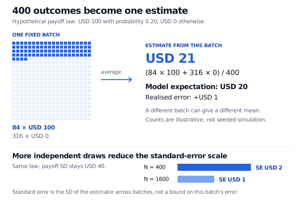
This fixed illustrative batch is a possible outcome, not a reported simulation or market dataset. Its realised error is USD 1. The true expectation remains USD 20; the estimator has not changed the model. Equivalently, the positive-payoff frequency 0.21 estimates 0.20; multiplying by USD 100 converts that probability estimate to a payoff estimate.
A fixed hypothetical batch has 84 payoffs of USD 100 and 316 zeros, producing a USD 21 estimate against a USD 20 target. With the same payoff law, theoretical standard error is USD 2 at 400 independent draws and USD 1 at 1600.
Original hypothetical example. Each square represents one output; blue squares pay USD 100. The lower bars compare theoretical standard errors, not confidence intervals or realised-error bounds.
Attach uncertainty to the estimator
With finite payoff variance σY2, independence gives
Var(θ^N)=NσY2,SE(θ^N)=NσY.
Here an individual payoff has standard deviation USD 40. The standard error of the average is USD 2 at N=400, falling to USD 1 at N=1600. Quadrupling the number of independent draws halves this uncertainty scale. It does not guarantee that the next realised error halves, or even gets smaller.
Usually σY is unknown. For N≥2, calculate sample variance with divisor N−1:
sY2=N−11i=1∑N(Yi−θ^N)2,SE=NsY.
For the 84-positive batch, this gives an estimated SE of approximately USD 2.0391. The Bernoulli plug-in convention instead substitutes p^=84/400=0.21 into the population variance formula, giving 100p^(1−p^)/400≈2.0365 USD. That uses divisor N for payoff variance. Both converge to the same scale; the first convention applies the finite-sample variance correction. Neither estimated SE is the observed USD 1 error.
For large enough samples with nonzero finite variance, the central limit theorem motivates the approximate fixed-sample interval θ^N±1.96SE at 95% confidence. Coverage describes repeated independent batches. It is not a range for an individual payoff. In sparse Bernoulli problems, use a suitable binomial interval: zero observed successes do not establish zero uncertainty.
For a fuller implementation, Simulation and Resampling develops the estimator and seeded code. The full lesson requires membership; its public preview shows the scope and prerequisites.
What more draws cannot repair
The sampling error above is conditional on the distribution being simulated. An incorrect model, miscalibrated inputs, a biased time discretisation or a coding error can leave an estimator precisely centred on the wrong target. A small standard error does not validate that target.
Dependence also changes the calculation. If every supposedly new draw simply repeats the first payoff, the average equals that single payoff and retains its USD 40 standard deviation. Independent draws are what justify dividing variance by N. Methods such as variance reduction can improve the estimator itself; their error calculation must respect how independent sampling units were constructed.
Sources
Paul Glasserman, Monte Carlo Methods in Financial Engineering (Springer, 2003), §§1.1.1–1.1.2: sample averages, sampling error and discounted-payoff estimation. Publisher record.
Mike Giles, Monte Carlo Methods, Lecture 1, slides 7–10 and 23: payoff averages, the CLT, empirical variance and variance of an independent average. Oxford lecture notes.