Monte Carlo standard error: Definition & Examples

Monte Carlo standard error is the standard deviation of a simulation estimator across hypothetical independent repetitions of the entire calculation. It measures the sampling noise introduced by using finitely many random draws. For a Monte Carlo estimator that averages independent, identically distributed outputs, it is the output standard deviation divided by the square root of the sample count.

An option-pricing engine may produce widely scattered simulated payoffs while estimating their average quite precisely. The payoff standard deviation describes that scatter; the standard error describes uncertainty in the estimated average. Neither measures whether the pricing model fits the market.

Calculate it from the outputs you actually average

Let $Y_1,\ldots,Y_N$ be independent outputs with a common distribution, mean $\mu$ and finite variance $\sigma_Y^2$ . Then

\hat\mu_N=\frac{1}{N}\sum_{i=1}^N Y_i, \qquad \text{SE}(\hat\mu_N)=\sqrt{\text{Var}(\hat\mu_N)} =\frac{\sigma_Y}{\sqrt N}.

The variance identity is exact: independence removes the cross-covariances, leaving $N\sigma_Y^2/N^2$ . A normal approximation is not needed to define standard error. When the population standard deviation is unknown, estimate it from the simulated outputs:

s_Y^2=\frac{1}{N-1}\sum_{i=1}^N(Y_i-\hat\mu_N)^2, \qquad \widehat{\text{SE}}(\hat\mu_N)=\frac{s_Y}{\sqrt N}, \qquad N\ge 2.

Here

s_Y

is a sample standard deviation, and

s_Y/\sqrt N

is an estimated standard error. Both have the same units as the quantity being averaged. The sample variance uses

N-1

; that does not turn the standard error's denominator into

\sqrt{N-1}

For risk-neutral option pricing with constant continuously compounded rate

r

and maturity

T

, take

Y_i=e^{-rT}H_i

, the discounted payoff on simulation

i

. Compute the standard deviation of these discounted payoffs. If instead you compute the standard deviation of the undiscounted

H_i

, multiply its standard error by

e^{-rT}

too. With stochastic discounting, average and analyse the pathwise discounted outputs directly. Glasserman develops this error accounting in §§1.1.1–1.1.2.

Four payoffs, three different numbers

Suppose four independent model simulations produce these stipulated discounted payoffs, in USD per unit of a hypothetical claim:

Simulation	1	2	3	4
Discounted payoff	0	0	4	8

Their average is USD 3. The squared deviations from that average sum to $9+9+1+25=44$ , giving

s_Y^2=\frac{44}{3}\ \text{USD}^2, \qquad s_Y\approx\text{USD }3.82971, \qquad \widehat{\text{SE}}=\frac{s_Y}{2} =\sqrt{\frac{11}{3}}\ \text{USD} \approx\text{USD }1.91485.

The report is therefore estimate USD 3; estimated SE USD 1.91485; four independent observations. The SE is neither the observed pricing error nor a guaranteed upper bound on it. The model's exact expectation has not been supplied, so the realised error cannot be calculated here. Four observations also give a fragile estimate of the payoff variance; they do not establish a reliable normal confidence interval.

A precision budget, not a promise about the next run

For a fixed output distribution, standard error falls as

N^{-1/2}

. Suppose a different hypothetical discounted-payoff distribution has a known standard deviation of USD 12:

Independent samples	Standard error, USD
2,500	0.24
10,000	0.12
40,000	0.06

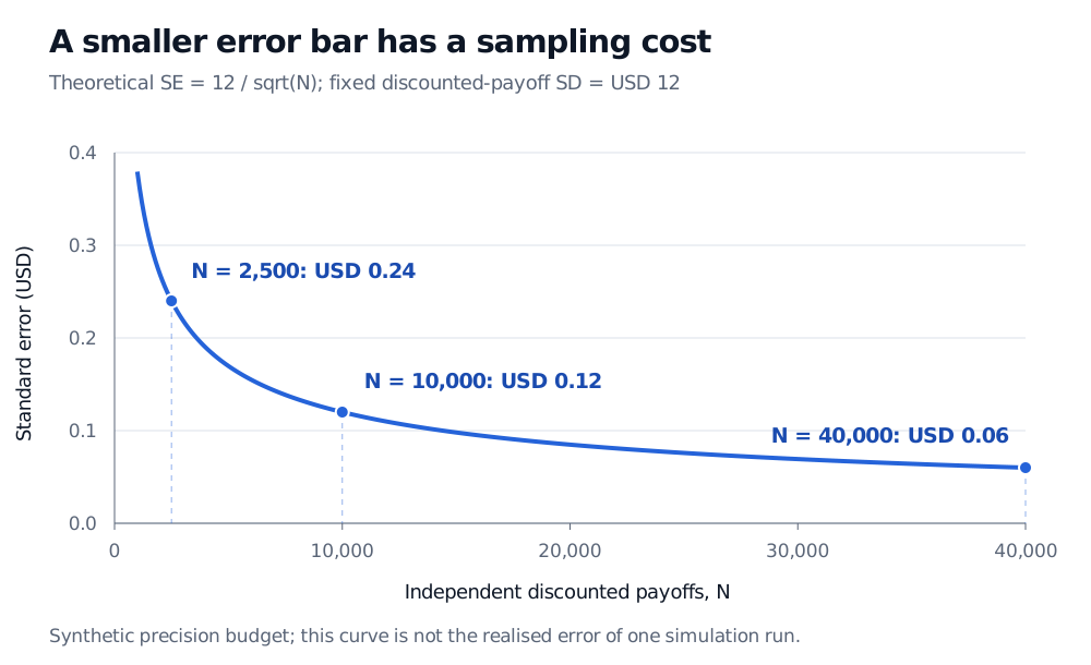
Theoretical Monte Carlo standard error with fixed discounted-payoff standard deviation USD 12: 2,500 independent samples give SE USD 0.24; 10,000 give USD 0.12; 40,000 give USD 0.06. Four times the samples halve standard error.

Original synthetic precision budget. The curve shows theoretical standard error under a fixed payoff distribution, not the realised error along a simulation run.

Halving standard error requires four times as many independent outputs. A particular estimate can nevertheless move farther from the target when more samples arrive. Variance reduction attacks the numerator instead: lowering the output standard deviation can save substantial computation without increasing $N$ .

A target SE also differs from a target confidence-interval half-width. With sufficiently accurate central-limit-theorem approximation, an approximate 95% interval is

\hat\mu_N\pm1.96\,\widehat{\text{SE}}.

For the USD 12 standard deviation, an SE of USD 0.06 needs 40,000 samples. At that count, the approximate 95% half-width is USD 0.1176. Targeting a half-width of USD 0.06 instead requires approximately $(1.96\times12/0.06)^2=153{,}664$ samples. If the standard deviation comes from a pilot estimate, these are planning estimates rather than guaranteed budgets.

A confidence interval describes repeated-sampling coverage under its assumptions: about 95% of intervals constructed by a valid 95% procedure cover the fixed target. It does not guarantee that this run's interval contains the target. Strong skewness, rare payoffs or heavy tails can make the normal approximation poor even when the sample count looks large. Shalizi's Monte Carlo notes, §§3–4, explain the expectation-estimation formula and why dependence changes it.

Count independent units; separate the other errors

With antithetic sampling, a draw and its mirror deliberately produce dependent payoff legs. For

M

independent pairs, form

A_j=(Y_j+Y_j^-)/2

and report

s_A/\sqrt M

. Compute

s_A

across the pair averages. Treating all

2M

legs as independent discards the covariance that the method was designed to create. Glasserman §4.2 derives this pair-level calculation.

Other designs need their own error analysis. Markov chain Monte Carlo has serial dependence; a deterministic low-discrepancy point set has no ordinary sampling distribution across random draws. Do not attach the independent-output formula solely because a program produced $N$ values.

Finally, an SE quantifies noise around the expectation of the implemented estimator. It excludes errors from an inappropriate model, uncertain calibrated parameters, missed barrier crossings or a coarse time-discretisation scheme. More paths can make a biased calculation look extremely precise. A sample SD of zero can also arise because no rare payoff has yet appeared; it does not establish that the model payoff is deterministic.

For a worked implementation that distinguishes simulation noise from uncertainty in observed data, see Simulation and Resampling, especially “Monte Carlo estimation and CLT error.” The full lesson requires membership; the public link provides its preview.

Sources

Paul Glasserman, Monte Carlo Methods in Financial Engineering, Springer, 2003, §§1.1.1–1.1.2 for Monte Carlo standard error and discounted-payoff estimation; §4.2, equations 4.27–4.28, for independent antithetic pair averages. Publisher's book page.
Cosma Rohilla Shalizi, Approximating Probabilities and Expectations by Repeated Simulation, or, “Monte Carlo”, Carnegie Mellon University, 36-402, 28 January 2025, §§3–4 — standard error of expectation estimates and dependent simulations.

Calculate it from the outputs you actually average

Four payoffs, three different numbers

A precision budget, not a promise about the next run

Count independent units; separate the other errors

Sources

Related terms

Central limit theorem

Confidence interval

Risk-neutral valuation

Standard deviation