A reverse discounted cash flow (reverse DCF) starts from a market value and solves for an input that makes a discounted cash flow model reproduce that value. The implied input gives an analyst a benchmark for assessing an independent operating forecast. Its interpretation depends on the model and the other inputs held fixed. Mauboussin and Rappaport, Expectations Investing tutorial 8
What cash flow would support a value of 200 million?
Suppose a fictional company's market-implied enterprise value is USD 200 million. If starting from a share price, multiply by shares outstanding to get common equity value, add debt and other financing claims, and subtract excess cash and other non-operating assets excluded from the cash flow forecast. This puts the market value on the same basis as free cash flow to the firm (FCFF), which is available to the firm's capital providers before financing payments. Mauboussin and Rappaport, tutorial 8, steps 1–3
Assume the business is already in steady state. The first FCFF arrives one year from today, then grows at a constant annual rate forever. Use a constant annual effective weighted average cost of capital (WACC) above . Both rates and the cash flows are nominal and use the same currency basis. Rearrange the Gordon growth model to solve for the first-year cash flow. Damodaran, chapter 15, Stable Growth Firm
At 9% WACC and 3% growth, the implied first cash flow is million. The same enterprise value implies 16 million at 11% WACC and 3% growth, or 8 million at 9% WACC and 5% growth. A higher discount rate requires more initial cash at the same growth rate. Faster growth lets later cash flows do more of the work.
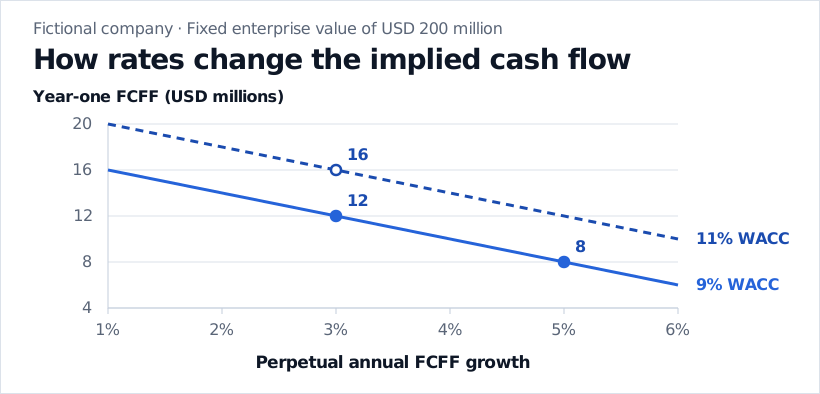
Every point on either line reproduces the same USD 200 million enterprise value under its own pair of rates.
If you instead have a first-year cash flow estimate and keep WACC fixed, the same equation gives implied growth . One observed price gives one equation. To infer more than one input, you need extra assumptions or evidence.
Check what the business would have to earn
In the 3% growth case, suppose each new dollar of invested capital earns a steady 12%. If growth comes from reinvestment at that return, the business must reinvest of after-tax operating profit each year. To leave 12 million in year-one FCFF, it would therefore need million in year-one after-tax operating profit. An independent forecast of 14 million under those same assumptions would leave 10.5 million in cash and support an enterprise value of 175 million. The comparison identifies an operating profit hurdle you can assess against margins and sales. If you change the growth assumption, rebuild the reinvestment forecast alongside it. Damodaran, chapter 15, Stable Growth Firm
When the company is still changing quickly, a model with an explicit forecast and a terminal value can be more informative. For example, hold the forecast margins, reinvestment policy, discount rate and mature growth assumptions fixed, then solve for how long the higher-growth phase must last to reproduce the market value. Test that duration against the competitive conditions that could sustain it. Mauboussin and Rappaport, tutorial 8, step 4
Section 1 of the SelfMadeQuant lesson shows the same inversion in an equity model. It fixes market price and forecast dividends to infer a return. The preview is public and the full lesson requires membership. Equity Valuation: Dividend Discount and DCF Models
Sources
- Michael J. Mauboussin and Alfred Rappaport, How Do You Perform a Price-Implied Expectations (PIE) Analysis?
- Aswath Damodaran, Investment Valuation, chapter 15, Stable Growth Firm.