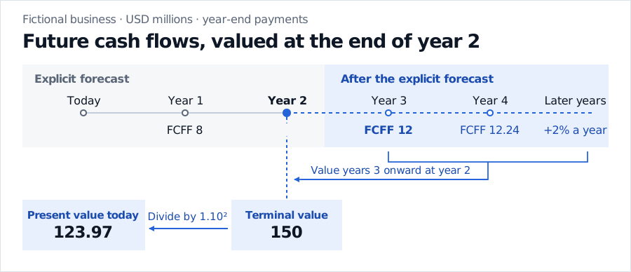
Suppose a fictional business generates free cash flow to the firm (FCFF) of USD 8 million in year one and USD 10 million in year two. At the end of year three, the first year beyond the explicit forecast, FCFF is expected to be USD 12 million. Assume it grows at 2% a year thereafter and the annual weighted average cost of capital (WACC) is 10% throughout. All payments are at year-end and the amounts and rates are nominal.
The Gordon growth model sums the growing cash flows from year three onward. Its result sits one period before the first payment, so the terminal value is dated at the end of year two. In USD millions,
A fictional business has year-one and year-two cash flows of USD 8 and 10 million. Year-three cash flow of USD 12 million and subsequent cash flows give a terminal value of USD 150 million at year two, worth USD 123.97 million today.
The year-two cash flow stays in the explicit forecast. The terminal value starts with the year-three cash flow and is discounted back two years.
At year two the model counts the explicit cash flow of 10 and the continuation value of 150 once each. Today's value of the operations is 8/1.10+(10+150)/1.102≈139.50 million. About 89% comes from the terminal component. Adding year three as a separate discounted payment would count it twice.
How much growth does the value assume?
Hold year-three FCFF fixed at 12 million and WACC at 10%. At 1% perpetual growth, year-two terminal value is 133.33 million. At 3%, it is 171.43 million. These changes come from year four onward. As growth approaches the discount rate, each successive discounted cash flow shrinks more slowly, and the series stops converging if g≥r for this positive cash flow stream.
For a business forecast, choose a perpetual growth rate the business can sustain relative to its market and match the growth and discount rates to the cash flows' currency and nominal or real basis. Then rebuild the first terminal cash flow to reflect the reinvestment that growth requires. In a stable-growth model with a constant return on new capital, the required share of after-tax operating profit reinvested is growth divided by that return. At a given return, faster growth requires a higher reinvestment share, which leaves less cash for investors and can offset the effect of the smaller denominator. Damodaran, Investment Valuation chapter 12 lecture notes
Compare an exit multiple on the same date
An exit multiple estimates what the business would be worth at the end of the explicit forecast based on a financial metric and a corresponding valuation multiple. Suppose year-two EBITDA is 20 million and the assumed exit multiple is 8 times trailing EBITDA. That gives an enterprise terminal value of 160 million at year two, so it receives the same two years of discounting as the perpetuity estimate. A forward multiple at that same date would use year-three EBITDA. The multiple and the metric need to use the same trailing or forward convention. Damodaran, Chapter 12 derivations, question 6
With the same 12 million first terminal FCFF and 10% WACC, a value of 160 million implies g=0.10−12/160=2.5% under the perpetuity model. That is one way to translate the difference into an assumption you can examine. A multiple drawn from comparable firms reflects how the market prices their growth, risk and profitability. A difference between the estimates can point to differences in those assumptions, in reinvestment, or in how EBITDA converts to cash flow.
For the equity version, section 4 of the SelfMadeQuant lesson uses the year-eight dividend to calculate terminal equity value at year seven. The preview is public, and the full lesson requires membership. Equity Valuation: Dividend Discount and DCF Models