A computational rule for turning a mathematical problem into a numerical answer, with explicit inputs, stopping criteria and assumptions.
Numerical method
A numerical method is a systematic procedure for solving a mathematical problem through calculations on numerical values, usually producing an approximation with a stated accuracy. In quant finance, it turns a pricing equation, an expectation or a risk model into something a computer can evaluate. The useful output is more than a number: it includes evidence that the calculation has met an appropriate stopping test.
For example, a market price may be observed while the implied volatility that reproduces it is unknown. A root solver tries candidate volatilities against the pricing equation. The financial model specifies the equation; the numerical method specifies how to solve it. Solving that equation accurately does not establish that the model describes the market accurately.
What makes the calculation a method?
A reproducible numerical calculation answers four questions:
Part
What must be specified?
Inputs
The equation or data, units, admissible domain and initial values.
Rule
How the next candidate, grid or estimate is calculated.
Stop
Which accuracy test ends the calculation, and what happens if the budget runs out.
Assumptions
What makes the rule and any claimed error bound valid.
Different problems need different rules. Root-finding solves equations; numerical integration approximates integrals; Monte Carlo simulation estimates quantities through sampled outcomes. A method may use a fixed grid rather than an iterative loop. Its accuracy might come with a deterministic bound, an asymptotic estimate or a statistical uncertainty measure; those are different kinds of evidence.
This dimensionless teaching example has a known positive root, 2, so the answer can be checked independently. In a pricing application the root would usually be an unknown parameter.
The function is continuous and its endpoint values have opposite signs. Test the midpoint and retain the half whose endpoint signs differ. Count each such replacement as one bracket update:
Completed update
Midpoint just tested
Its residual f(x)
Retained bracket
1
1.5
0.25
[1,1.5]
2
1.25
−0.4375
[1.25,1.5]
3
1.375
−0.109375
[1.375,1.5]
Our return convention is to take the new bracket's midpoint. After three updates this gives
A stopping rule requiring a midpoint error bound no larger than 0.0625 is now satisfied. The bound comes from the retained interval, without knowing the exact root. For this checkable example, the actual error is approximately 0.0232864376, smaller than the bound.
The last midpoint tested during the three updates was 1.375; the returned new midpoint is 1.4375. Forming that final midpoint needs no additional function evaluation. If its residual is also wanted, evaluate it separately. Counting updates, evaluations and returned estimates as though they were interchangeable makes apparently identical algorithms disagree.
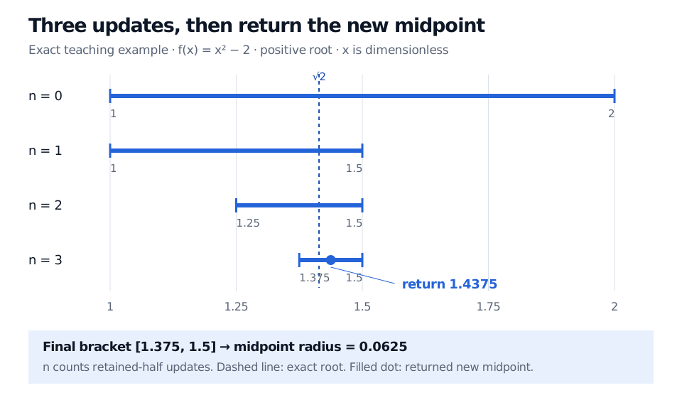
Four retained bisection intervals shrink from [1, 2] to [1.375, 1.5]. The returned new midpoint is 1.4375 and its midpoint error bound is 0.0625. A dashed line marks the positive square root of two.
Original exact-arithmetic teaching diagram. All horizontal values are dimensionless; the filled dot is the returned midpoint after three retained-half updates.
The stopping message matters
The bisection bound needs continuity and trustworthy endpoint signs throughout the retained bracket. Opposite signs alone are insufficient: 1/(x−1) changes sign between zero and two but has a pole there and no zero. In floating-point arithmetic, a midpoint can also round to an endpoint, preventing further progress. A useful implementation reports that limit or an exhausted evaluation budget instead of silently treating it as success.
Nor does a small equation residual automatically mean a small parameter error. For g(x)=10−12(x−1), the residual at zero is −10−12 while the distance to the root is one. Choose tolerances in the units of the quantity being controlled. A pricing residual in currency and an error in decimal volatility need separate interpretation.
Numerical analysis studies why these methods work, how errors behave and which procedures are reliable. For a financial continuation, the Root-Finding and Numerical Integration lesson formulates a bond-yield equation and an expectation integral. The public page provides a preview; the full lesson requires membership.
Sources
John V. Guttag, Introduction to Computation and Programming Using Python: With Application to Understanding Data, 2nd ed., MIT Press, copyright 2016, §3.3, pp. 30–34: approximation specifications and bisection search.
SciPy: bisect: continuity, sign requirements, parameter tolerances and convergence reporting. The worked ledger here states its own return convention rather than reproducing a particular library's trace.