Numerical integration turns an integral into weighted function values. Compare four cash-flow approximations and distinguish sampling, discretisation and model error.
Numerical integration
Numerical integration, also called quadrature, computes an approximation to a definite integral from values of its integrand. Instead of finding a symbolic antiderivative, it combines sampled values with weights:
I=∫abf(x)dx≈Q=j=1∑mwjf(xj).
The nodes xj say where to evaluate the function; the weights wj say how much each value contributes. In this convention the weights include interval widths. If f is a cash rate in USD/year and x is time in years, Q is an amount in USD.
For quants, this is a practical bridge from an expectation, probability or continuous cash-flow model to a number. The integral specifies the quantity being valued; the numerical rule specifies how to calculate it.
A cash rate is not a cash amount
Suppose a synthetic project receives cash continuously at rate
c(t)=2+6t,
where t is measured in years and c(t) in thousand USD/year, over 0≤t≤3. This is an illustrative deterministic model, with no discounting. The total receipt is the rate integrated over time, not the sum of the rate observations.
Split the horizon into three one-year intervals. The four endpoint rates are 2,8,14,20. Different choices of representative height give different totals:
Rule
Calculation in thousand USD
Total receipt
Left endpoint rectangles
1(2+8+14)=24
USD 24,000
Right endpoint rectangles
1(8+14+20)=42
USD 42,000
Midpoint rectangles
1(5+11+17)=33
USD 33,000
Trapezoids
1(2/2+8+14+20/2)=33
USD 33,000
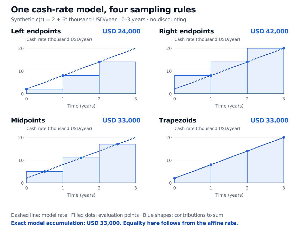
Four quadrature constructions for a synthetic cash rate rising from 2 to 20 thousand USD/year over three years. Left rectangles total USD 24,000; right rectangles USD 42,000; midpoint rectangles and trapezoids each USD 33,000.
Original synthetic model. Each shaded piece contributes rate times time. Midpoint rectangles balance the linear rise within each year; trapezoids follow it exactly. Both reproduce the USD 33,000 integral.
An independent check uses geometry: a rectangle of height 2 over three years contributes 6 thousand USD, and the triangle above it contributes 18×3/2=27 thousand USD. Together they give 33 thousand USD. Equivalently,
∫03(2+6t)dt=[2t+3t2]03=33.
Midpoint and trapezoid rules are exact for this affine rate. Their agreement here says nothing about their accuracy for an arbitrary curved rate. If only the four endpoint observations were known, assuming straight lines between them would be an interpolation choice: other curves through those same observations can have different integrals. Midpoint evaluation additionally needs the three interior values.
Choose the rule around the information available
If the function can be evaluated at new points, you can refine the grid, compare resolutions, or use adaptive quadrature to concentrate work where the integrand is difficult. Gaussian quadrature chooses nodes and weights to achieve high polynomial exactness with relatively few evaluations. These are choices about the numerical calculation, rather than changes to the model.
If only stored samples are available, additional midpoint or Gaussian-node values are not free observations. A trapezoid calculation integrates the piecewise straight-line interpolant through the supplied samples. Refining that interpolant with invented intermediate points does not create information about the unknown curve.
Applying a local rule repeatedly across a partition is composite quadrature. For curved functions, comparing successive partitions is useful evidence of convergence, but two nearby answers alone are not a certified error bound. Narrow features can fall between sampled nodes. An adaptive integrator's reported error is an estimate, not a guarantee that the financial model is correct.
Keep the errors separate
A quadrature calculation can be very accurate for the wrong integrand. For an expected payoff, both the payoff and its probability density belong in the integrand. Discounting belongs there too when computing present value rather than undiscounted receipts. Negative contributions must keep their signs: an integral measures net accumulation, not necessarily geometric area.
A finite integration window also omits any contribution outside it. Adding more nodes inside that window can reduce discretisation error while leaving tail truncation error untouched. Roundoff, noisy input data and model assumptions are further limits; increasing the panel count does not remove them all.
The SelfMadeQuant lesson Root-Finding and Numerical Integration develops the composite trapezoid formula and connects it to expectations and pricing. Its preview is public; the full lesson requires membership.
Sources
James Stewart, Single Variable Calculus: Early Transcendentals, 6th edition, Thomson Brooks/Cole, 2008, §7.7, “Approximate Integration”: endpoint, midpoint and trapezoid approximations; numerical integration from function values or collected data.