Gaussian quadrature chooses nodes and weights for polynomial exactness. Derive the two-point Gauss–Legendre rule, map its interval and see its first failure.
Gaussian quadrature
Gaussian quadrature is a family of numerical integration rules that chooses both sampling locations and weights to integrate polynomials of the highest possible degree for a given number of evaluations. An n-point Gaussian rule is exact through degree 2n−1, for its specified interval and weight function, in exact arithmetic.
That economy matters when evaluating an integrand is expensive: one value may itself require a pricing calculation. But polynomial exactness is a property of the integration rule. It does not validate the payoff, probability model or market inputs being integrated.
Moving the sample points
The most familiar case is Gauss–Legendre quadrature, for an ordinary, unweighted definite integral on a finite interval. On [−1,1], its two-point rule is
∫−11f(t)dt≈f(−31)+f(31).
Neither sample is an endpoint or the midpoint. To see where these points come from, impose symmetry: take nodes −c,c and equal weights w. Exactness for the constant function gives 2w=2, hence w=1. Exactness for t2 then requires 2c2=2/3, hence c=1/3. Odd powers through the cubic integrate to zero and their weighted values cancel. The rule therefore integrates every cubic, not just the four individual monomials.
More generally, the Gauss–Legendre nodes are the roots of the degree-n Legendre polynomial. Those polynomials are orthogonal under integration on [−1,1]. This is why a carefully selected set of nodes can deliver more polynomial exactness than arbitrary fixed nodes with weights alone. Polynomial interpolation supplies the underlying connection between sampled values and integrated polynomials.
Two values on zero to one
Changing intervals also changes the weights. With
x=2a+b+2b−at,dx=2b−adt,
the mapped rule is
Qn=2b−ai=1∑nwif(2a+b+2b−ati).
The factor (b−a)/2 is essential. For [0,1], the two sample locations and their mapped weights are
Take two synthetic dimensionless functions. Use the actual irrational nodes, rather than their rounded labels:
Integrand
Two-point estimate Q2
Exact integral I
Signed error Q2−I
x3
1/4
1/4
0
x4
7/36≈0.194444444
1/5=0.2
−1/180≈−0.005555556
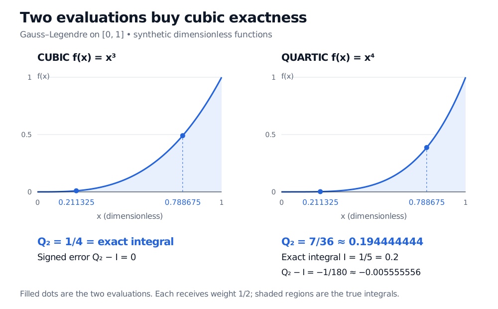
Two-point Gauss–Legendre on zero to one samples 0.211325 and 0.788675 with weight one half each. The cubic integral is exactly one quarter; the quartic estimate seven thirty-sixths understates one fifth by one one-hundred-eightieth.
Original dimensionless benchmark. The same two nodes integrate the cubic exactly but miss the quartic. Filled dots show evaluated values; shaded areas show the true integrals.
The cubic result does not mean that two points reconstruct the whole cubic curve. They recover its integral. The quartic is the first degree outside this rule's exactness guarantee; three-point Gauss–Legendre would integrate that quartic exactly. Floating-point calculations should report agreement within a stated tolerance, even for a mathematically exact case.
Match the rule to the integral
“Gaussian” here refers to Gauss's quadrature construction, not an assumption that the variable follows a normal distribution. Gauss–Legendre uses weight function 1 on [−1,1]. Gauss–Hermite instead uses the weight e−t2 on the whole real line. Their nodes and weights cannot be exchanged unchanged. Normal expectations require the appropriate density scaling and change of variables.
For a finite-support continuous model, an expected value has the form
E[g(X)]=∫abg(x)p(x)dx.
Applying Gauss–Legendre here means evaluating the entire product g(x)p(x). Cubic exactness concerns that product, not the payoff g alone. If the original distribution has infinite support, cutting the domain to [a,b] introduces a separate tail-truncation error.
Smooth integrands often suit Gaussian rules. A payoff kink, discontinuity or singularity deserves attention before increasing the order: splitting at a known feature or choosing a rule adapted to the weight may work better. Composite quadrature describes interval subdivision and can also be combined with local Gaussian rules. A higher polynomial degree of exactness is no universal accuracy ranking across all integrands.
For the financial expectation setup and a transparent trapezoid baseline, read Root-Finding and Numerical Integration (public preview; full lesson requires membership).
Sources
Lloyd N. Trefethen and David Bau III, Numerical Linear Algebra (SIAM, 1997), Lecture 37, pp. 289–290: polynomial exactness, orthogonality and the Gauss–Legendre construction.