Understand what makes a numerical answer reliable: problem conditioning, algorithm stability, approximation error, rounding and computational cost.
Numerical analysis
Numerical analysis is the study and design of computational algorithms for mathematical problems involving real or complex quantities. It asks how to obtain useful answers with finite time, memory and precision, and how to establish their accuracy, convergence and reliability. Pricing an option on a grid, fitting a regression and estimating a Greek all require these judgments.
A numerical method supplies the computational steps. Numerical analysis explains when those steps work, what errors they introduce and how much computation is needed. Its scope includes solving equations, integration, differentiation, optimisation, interpolation and differential equations; controlling rounding is one part of the subject.
Four questions behind one number
Suppose a pricing routine returns a value. Before trusting more displayed digits, separate four questions:
Question
What it diagnoses
A possible response
Would a small change in the supplied data substantially change the exact answer?
Use a suitable precision and arithmetic implementation, then check the result
These questions interact. Rounding creates perturbations; algorithmic stability describes how the computation handles them; conditioning determines how strongly the underlying problem responds. A finer grid changes approximation error, yet can increase work and expose other numerical difficulties. More precision cannot recover an unknown market input or repair an inappropriate financial model.
A sensitive answer with no rounding at all
Take the dimensionless toy map
f(x)=1−x1,x=1.
This is an illustration of sensitivity, not a calibrated pricing formula. At x=0.99, the exact answer is 100. Change the input to 0.9901 and the exact answer becomes
f(0.9901)=9910000≈101.010101.
Measured relative to the original values, the changes are
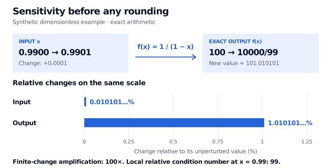
The relative output change is exactly 100 times the relative input change for this particular finite perturbation. There is no algorithmic failure in these exact calculations: the problem itself amplifies the input change.
Exact dimensionless inputs 0.9900 and 0.9901 give outputs 100 and 10000/99. Relative input change 0.010101 percent becomes relative output change 1.010101 percent, a finite amplification of 100.
Original synthetic example in exact arithmetic. Both bars use the same percentage scale. The finite-change amplification is 100; the local relative condition number at the original input is 99.
For a differentiable scalar map with nonzero input and output, the local relative condition number is
κ(x)=f(x)xf′(x).
Here κ(0.99)=99. Multiplying that by the relative input change predicts a relative output change of 99/9900=0.01, or 1%. The exact change is slightly larger because a local derivative gives a first-order approximation, rather than an exact formula for a finite perturbation. Moving toward the pole at x=1 increases the sensitivity; at the pole the requested value is undefined.
What a quant should check
For a grid-based option price, vary the grid while keeping the financial model fixed. Study convergence and test boundaries or payoff kinks; one small difference between two grids is useful evidence, not a universal error certificate. For a linear hedge solve, test sensitivity to exposure changes separately from the solver's arithmetic. A stable solver can faithfully reveal that the available instruments nearly duplicate one another.
Choose an error scale that fits the decision. Absolute error measures a price discrepancy in currency units; relative error compares it with a nonzero reference value. Near a zero reference, relative error may be undefined or misleading. Compare against an analytic benchmark where available, an independent method or a carefully justified error bound. Record computational cost alongside accuracy: the useful method must meet both the numerical tolerance and the time budget.
For a fuller finance example, Numerical Conditioning and Stability connects these ideas to hedge ratios, regression and covariance calculations. Its full lesson requires membership; a public preview is available.
Sources
Lloyd N. Trefethen and David Bau III, Numerical Linear Algebra, SIAM, 1997. Appendix, “The Definition of Numerical Analysis,” pp. 321–324; Lectures 12–14 on conditioning, floating-point arithmetic and stability.
David Bindel, Cornell CS 4220, “Background Plus a Bit”, Spring 2020, §6, “Sensitivity, conditioning, and types of error.”