The Laplace distribution has a sharp peak and exponential tails. Compare log-return tail probabilities with a variance-matched Gaussian and connect Laplace noise to absolute-error loss.
Laplace distribution
The Laplace distribution, also called the double exponential distribution, is a symmetric continuous probability distribution with a sharp central peak and exponentially decaying tails. It gives more weight to sufficiently extreme outcomes than a normal distribution with the same variance. In finance, it is a simple alternative model for return shocks or regression residuals when a Gaussian assumption puts too little probability on large moves.
Both parameters have the same units as X. The mean, median and mode equal μ, while
Var(X)=2b2,SD(X)=2b.
Scale is not standard deviation. Setting b=1% does not give a 1% standard deviation; it gives approximately 1.4142%. The density is continuous at its peak, though its slope changes abruptly there. The peak is not an atom: P(X=μ)=0. NIST's distribution reference gives this location-scale parameterisation.
Same volatility, different risk story
Suppose a researcher models a synthetic one-period log return as X=log(S1/S0)∼Laplace(0,0.01). The period is fixed; the scale is 0.01 in decimal log-return units. This is a modelling exercise, not a fit to observed prices or a risk-neutral pricing assumption.
The variance is 0.0002 and the standard deviation is approximately 0.014142, or 1.4142 percentage points. Compare it with Z∼N(0,0.0002): the same centre and variance, with a different distributional shape.
For any a≥0, integrating both Laplace tails gives a particularly simple result:
P(∣X∣>a)=2∫a∞2b1e−x/bdx=e−a/b.
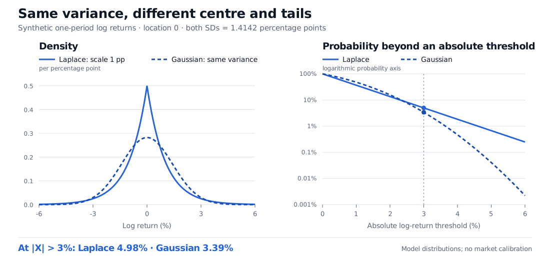
At an absolute log return of 3%, this probability is e−3≈4.98%. The variance-matched Gaussian assigns approximately 3.39% to the same event. These are two-sided probabilities; the Laplace downside probability alone is half of 4.98%.
Absolute log-return threshold
Laplace probability beyond it
Matched-variance normal
1%
36.79%
47.95%
3%
4.98%
3.39%
5%
0.67%
0.04%
Synthetic one-period log-return comparison: both models have mean zero and standard deviation 1.4142 percentage points. Laplace scale is 1 percentage point, and its density peaks at 0.5 per percentage point. Beyond an absolute log return of 3%, Laplace probability is 4.98% and matched-variance Gaussian probability is 3.39%.
Original synthetic model comparison. Left: density per percentage point. Right: two-sided exceedance probability on a logarithmic vertical axis; the straight Laplace tail reflects exponential decay. Visible plotting ranges do not truncate either distribution.
The 1% row matters: “heavier tails” does not mean a larger exceedance probability at every threshold. The Laplace model puts more mass very near zero, less at intermediate distances and more sufficiently far out. Equal variance alone cannot settle a tail-risk comparison.
Log returns also keep S1=S0eX positive despite the unbounded support. A log return of minus 3% corresponds to a simple return e−0.03−1, rather than exactly minus 3%. Zero mean log return means median terminal price S0; it does not imply zero expected simple return.
Exponential tails are still light tails
“Heavy” needs a reference. Laplace tails are heavier than Gaussian tails, whose decay includes a quadratic exponent. They are not power-law tails, and they are light-tailed under the exponential-moment definition of heavy-tailed distributions.
To see why, split the density at its centre. The moment-generating function is
E[etX]=2eμt(1−bt1+1+bt1)=1−b2t2eμt,∣t∣<1/b.
It is finite in a neighbourhood of zero. All positive integer absolute central moments are finite too: E[∣X−μ∣k]=k!bk. One quick explanation is that ∣X−μ∣ has an exponential distribution with mean b.
In the return example, b<1, so evaluating the MGF at t=1 gives E[eX]−1=1/(1−b2)−1≈0.010001%. This small positive expected simple return follows from exponentiation, despite zero mean log return. It is a model consequence, not a trading edge.
Why absolute error appears in estimation
For independent observations from a common Laplace model, the negative log-likelihood is
−ℓ(μ,b)=nlog(2b)+b1i=1∑n∣xi−μ∣.
At fixed positive b, maximum likelihood therefore minimises total absolute deviation. For a nonconstant sample, a sample median is a location estimate, and the fitted scale is the mean absolute deviation about that median, not the median absolute deviation. If every observation is identical, the likelihood has no finite maximiser with b>0; it grows as b approaches zero. With an even sample size, a median may be any point between the two middle order statistics. SciPy's distribution notes describe these estimators.
The same algebra explains regression with independent, common-scale Laplace residuals: maximising likelihood minimises the sum of absolute residuals. Doubling a residual doubles its contribution, whereas squared-error loss quadruples it. This reduces the direct penalty from large residuals; it does not make a regression immune to influential predictor values or model misspecification.
For that connection, The Probabilistic Interpretation of Least Squares develops the Gaussian likelihood and contrasts Laplace noise with absolute-error loss. The full lesson requires membership; a public preview is available.
A symmetric one-period Laplace law cannot by itself describe return skew, volatility clustering or dependence across assets. Nor does selecting it validate the estimated tail probabilities. Those require evidence about the data, horizon and intended use.
Sources
Dimitri P. Bertsekas and John N. Tsitsiklis, Introduction to Probability, 2nd edition, Athena Scientific, 2008: Chapter 3, §3.1 Problem 2, p.184; §4.1, pp.212–213, on the two-sided exponential law.