Understand constant proportional decrease, calculate half-life, and distinguish exponential decay from fixed losses, discounting and mean reversion.
Exponential decay
Exponential decay is a decrease at a constant rate relative to the amount currently remaining. Equal time intervals remove the same fraction, so the absolute amount lost becomes smaller as the quantity shrinks. A constant positive interest rate produces this shape in a discount factor as maturity increases.
For a positive initial quantity A0, the continuous model is
A(t)=A0e−kt,k>0,t≥0.
Here k is the decay constant, measured in inverse time: per year if t is in years. The exponent kt must be dimensionless. This is an exponential function with a negative time coefficient; reversing that sign gives exponential growth.
A percentage of the remainder
Suppose a synthetic quantity starts at 100 units and follows A(t)=100e−0.2t, with time in years. After one year it is about 81.873075 units; after five years,
A(5)=100e−1≈36.787944 units.
The rate k=0.2 per year does not mean losing 20 units each year, or even losing exactly 20% over a whole year. The one-year multiplier is e−0.2, so the one-year decrease is 1−e−0.2≈18.1269% of that year's starting amount. At the next anniversary the same percentage applies to a smaller base.
More generally, for any interval length Δ>0,
A(t)A(t+Δ)=e−kΔ.
This ratio is independent of the starting date t. If a discrete model instead specifies a fractional decrease d each period of length Δ, its multiplier is 1−d and the matching continuous rate is k=−ln(1−d)/Δ, for 0<d<1. The natural logarithm converts the observed multiplier into a rate.
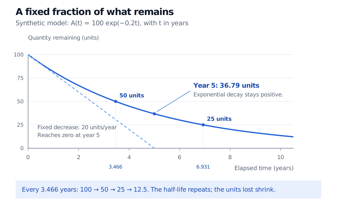
Synthetic decay from 100 units: the exponential curve has 50 units after 3.466 years, 25 after 6.931 years and 36.79 at year 5. A contrasting fixed decrease of 20 units per year reaches zero at year 5.
Original synthetic comparison. Both curves begin at 100 units with an initial slope of minus 20 units per year. Only the exponential curve keeps a constant proportional decay rate.
The calculus statement makes that distinction precise:
A′(t)=−kA(t),A(t)A′(t)=−k.
The slope is negative, but its magnitude shrinks with the remaining amount. Also A′′(t)=k2A(t)>0: the falling curve bends upward and becomes flatter. The fixed-decrease line 100−20t has constant slope and reaches zero at year five. Extending that line beyond year five would give negative quantities; it is a different model.
Half-life repeats
The half-lifeh is the time required to halve the remaining quantity. Solve A(t+h)/A(t)=1/2:
e−kh=21⟹h=kln2.
For the example, h=ln2/0.2≈3.465736 years. Starting from 100 units, successive half-lives leave 50, 25 and 12.5 units. The same duration halves each new remainder; it does not remove another 50 units.
For A0>0 and k>0, the model approaches zero as time grows without bound, but remains strictly positive at every finite time. A displayed zero caused by rounding is not a mathematical extinction date. If k=0 the level is constant; if k<0 the same formula describes growth instead of decay.
Discounting has this shape, with a different meaning
Under a constant continuously compounded annual rate r>0, the discount factor for maturity T years is D(0,T)=e−rT. The present value of a certain payment F is Fe−rT.
For an intentionally hypothetical flat rate of 20% per year, a payment of USD 100 due in five years has present value 100e−0.2(5)≈USD 36.79. The contractual payment is still USD 100. Comparing present values of equal payments at progressively later maturities produces a decay curve; it does not forecast an asset losing value through calendar time. The rate convention is continuous compounding, and a maturity-dependent rate curve need not produce this single constant-rate exponential. Negative constant rates reverse the direction.
A further distinction matters in mean reversion. In the deterministic equation x′(t)=−k(x(t)−m), the solution is
x(t)=m+(x(0)−m)e−kt.
It is the deviation from the equilibriumm whose magnitude decays exponentially. The level approaches m, which need not be zero. With random shocks, individual paths need not fall smoothly or reach a halfway level at the deterministic half-life. Choosing a decay constant is a modelling assumption, not evidence that market prices or trading signals actually follow that law.
To build the underlying algebra, Exponentials and Logarithms develops exponential multipliers and log rates. Time Value of Money compares discounting conventions and dated cash flows. Both offer public previews; full lessons require membership.
Sources
James Stewart, Single Variable Calculus: Early Transcendentals, 6th edition (2008), §3.8, “Exponential Growth and Decay,” pp. 234–238.
John C. Hull, Options, Futures, and Other Derivatives, 9th Global Edition, §4.2, “Measuring Interest Rates,” especially continuous compounding and equations (4.2)–(4.4).