Distinguish the Brownian noise loading from its variance rate and generator convention, with a price-versus-return GBM example and a checked one-day increment.
Diffusion coefficient
The diffusion coefficient is the loading on Brownian noise in a stochastic differential equation. It determines the local scale of random movement in the variable being modelled. For a stock price, that loading has price units; the familiar percentage volatility becomes a price diffusion only after multiplication by the current price.
This distinction prevents a practical simulation error: putting a 20% return volatility directly into a price equation does not produce a 20% return model.
where Wt is standard Brownian motion. Here a is the drift, and b is the diffusion coefficient. For a small interval of length h, freezing the coefficients at the current state gives the Euler approximation
ΔX≈a(t,Xt)h+b(t,Xt)hZ,Z∼N(0,1).
The noise standard deviation is ∣b∣h; its variance is b2h. The coefficient itself is neither the variance nor a finite-period standard deviation. If X is measured in USD and the clock in years, b has units USD/year, while b2 has units USD²/year.
Under suitable continuity and moment conditions, the local conditional variance satisfies
Var(Xt+h−Xt∣Ft)=b(t,Xt)2h+o(h),h↓0.
The remainder becomes negligible relative to h. This is a local statement, not a promise that every finite-horizon increment is Gaussian. The associated quadratic variation identity is
d[X]t=b(t,Xt)2dt.
It records accumulated path variation; it does not make b2h an exact conditional variance over an arbitrary future interval.
with time in years and current price St=100 USD. The return volatility parameter is σ=0.20 per square root year. The price diffusion is b(St)=σSt=20 USD/year, and the price's local variance rate is b(St)2=400 USD²/year.
For one model day, using h=1/252 year, the Euler increment is
ΔSEuler=2525+25220Z.
Quantity
One model day
Mean price increment
USD 0.01984
Noise standard deviation
USD 1.25988
Increment variance
1.58730 USD²
The 20 is a loading, the 400 is a rate, and the 1.25988 is a standard deviation over a specified interval. Confusing them changes both the units and the simulated risk.
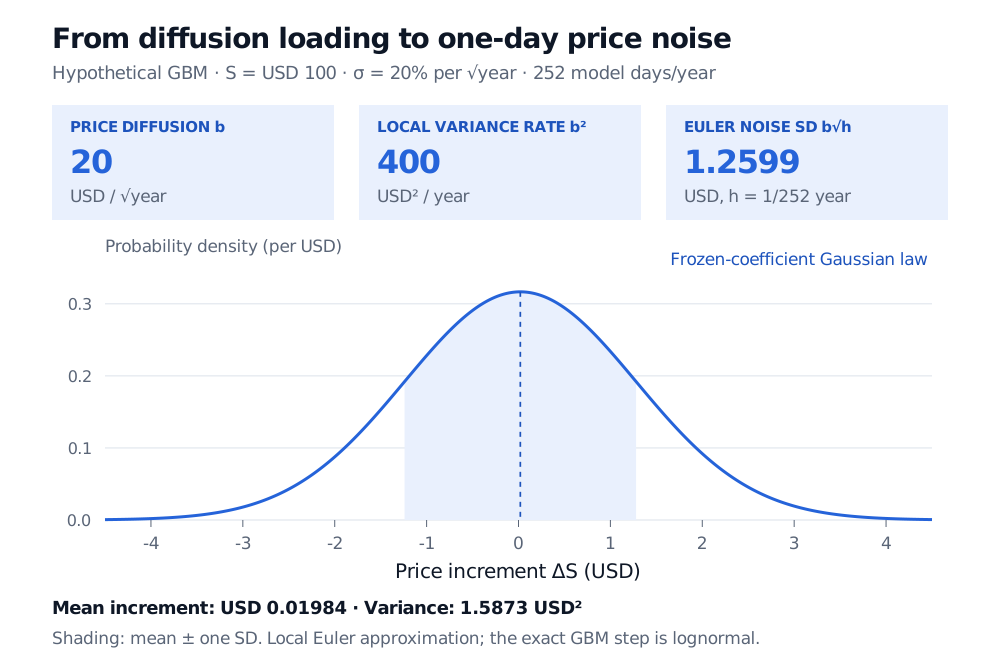
The frozen-coefficient one-model-day price increment has a Gaussian density with mean USD 0.01984, standard deviation USD 1.25988 and variance 1.58730 USD². Its price diffusion is 20 USD per square root year and its local variance rate is 400 USD² per year.
Original hypothetical model illustration. The shaded region is the Euler mean plus or minus one standard deviation, not a bound on price moves. A year contains 252 equal model days here.
Even for this simple model, local and exact finite-step variances differ. The exact conditional variance is
Var(St+h−St∣Ft)=St2e2μh(eσ2h−1),
which gives 1.58806 USD² for this day, compared with the Euler value 1.58730 USD². The gap is small here because the step is short. The exact price transition is lognormal; freezing the price-dependent loading produces the normal Euler increment shown above.
Why another source may call something else “diffusion”
Always check the equation. For a smooth function f, the scalar diffusion's generator is
Ltf(x)=a(t,x)f′(x)+21b(t,x)2f′′(x).
Thus the loading is b, the local variance rate is b2, and the coefficient on the second derivative is b2/2. A heat-equation convention that writes Df′′ uses D=b2/2. Transferring a number between these conventions without its defining equation can introduce a square or a factor-of-two error. Itô's lemma is what connects the noise loading to this curvature term.
For several state variables driven by independent standard Brownian factors, write dXt=adt+BdWt. The loading matrix is B, while the local covariance matrix is BB⊤; half of that matrix weights the generator's second derivatives. Some texts reserve “diffusion matrix” for BB⊤ and call B the dispersion matrix.
Finally, a scalar loading can be negative. Its sign disappears from the local variance, but it still specifies exposure to the named Brownian driver and can affect dependence with other variables driven by that same noise. Quoting only a variance rate discards that exposure information.
Sources
John C. Hull, Options, Futures, and Other Derivatives, 9th Global Edition (Pearson, 2018), §§14.2–14.3: Wiener scaling, variance rates, state-dependent Itô coefficients and proportional stock-price noise.
Ioannis Karatzas and Steven E. Shreve, Brownian Motion and Stochastic Calculus, first edition (Springer, 1988), Chapter 5, §2 equation (2.2) and §4 equation (4.1): dispersion versus diffusion matrices and the second-order operator.