A differential equation specifies a rule for an unknown function and its rates of change. Use a cash account to distinguish the rule, its solution family and an initial condition.
Differential equation
A differential equation is an equation involving an unknown function and one or more of its derivatives. It specifies a relationship between a quantity and its rates of change. Solving it means finding a function that satisfies that relationship throughout a stated domain.
For a quant, this changes the question from “What is the value now?” to “What rule connects the value to how it evolves?” A cash balance can grow at a rate proportional to its current size; an option value can be constrained by how it changes with time and the underlying price. The equation describes the rule. Additional information, such as a starting balance or an expiry payoff, helps select the relevant solution.
A rate is not a balance
Suppose a hypothetical cash account has USD 100 initially, earns a stipulated constant 4% continuously compounded annual rate, and has no deposits, withdrawals, fees or taxes. Let B(t) be its balance in USD, with t measured in years. Its rule is
B′(t)=0.04B(t),B(0)=100.
Here B′(t)=dB/dt is measured in USD per year. The coefficient 0.04 has units of inverse years, so both sides have the same units. Initially,
B′(0)=0.04×100=4USD per year.
This does not say that the account earns exactly USD 4 every year. As the balance grows, the same percentage rate acts on a larger amount. The straight line 100+4t has constant derivative 4; it therefore fails the differential equation once t>0.
Nor is 4% here an annual effective rate. The corresponding one-year percentage increase is e0.04−1≈4.08%. The compounding convention is part of the model, not a cosmetic label.
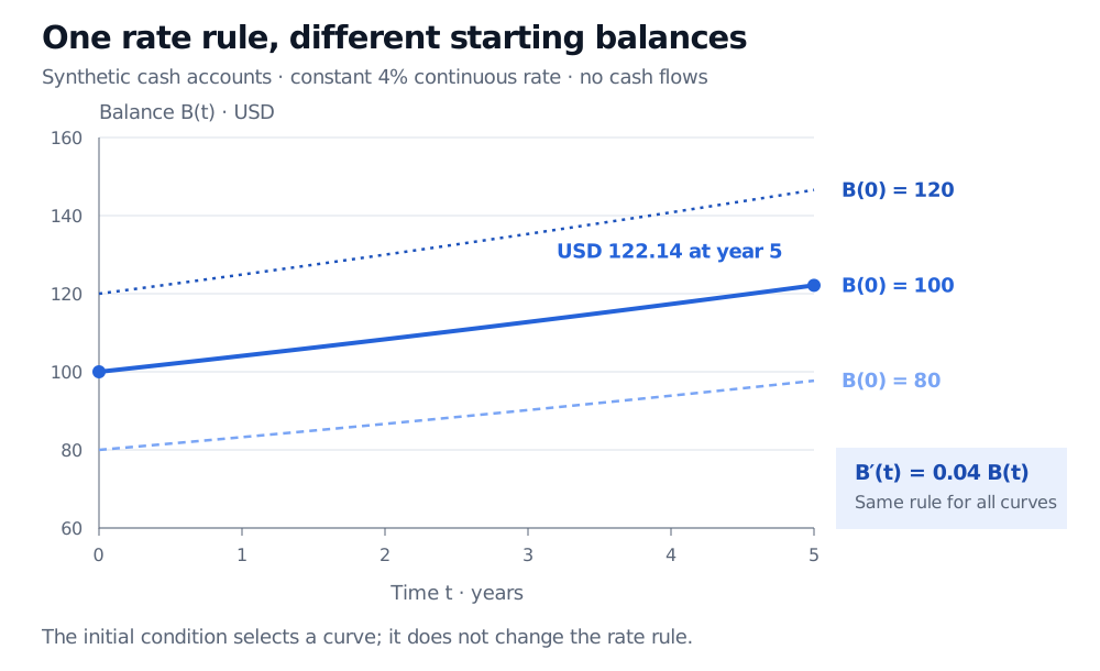
Thus the rate rule alone does not identify the account balance. Starting with USD 80 or USD 120 produces another solution of the same equation. For a nonnegative cash-balance model, take C≥0; C=0 gives the zero balance throughout.
The initial conditionB(0)=100 fixes C=100, selecting
B(t)=100e0.04t.
Together, the differential equation and starting value form an initial-value problem. For this equation the selected solution exists and is unique for all t≥0. Existence and uniqueness are mathematical properties to check in more general problems; writing down an initial condition does not automatically guarantee either.
Three synthetic cash-account solutions of B prime equals 0.04B, with time in years. Initial balances USD 80, USD 100 and USD 120 select different exponential curves. The solid blue curve starts at USD 100 and reaches USD 122.14 after five years.
Original deterministic model comparison: the same constant 4% continuous rate applies to all three starting balances, with no cash flows. The initial condition selects the curve.
At five years,
B(5)=100e0.2≈122.1402758USD.
The balance is USD 122.14 rounded to cents, while the instantaneous growth rate is about USD 4.89 per year. These are different quantities. The result follows from the stipulated rate; it is not a forecast of an investment return or a claim that an actual account offers these terms.
There are two separate checks on a proposed solution: substitute its derivative into the equation, then test the initial condition. For example, 120e0.04t passes the first check but fails the second. Merely matching the starting point is also insufficient: 100+4t starts correctly but fails the rate rule.
Which kind of equation is being used?
The term covers several settings that need different mathematics:
Setting
Unknown and derivatives
Quant-finance use
Ordinary differential equation, or ODE
A function of one independent variable, such as B(t) and its time derivative
Deterministic cash accumulation or a deterministic mean-reversion rule
Partial differential equation, or PDE
A function of several independent variables, with partial derivatives, such as option value V(S,t)
The Black-Scholes model relates changes in value across time and underlying price under its pricing assumptions
A stochastic process driven by specified random increments
A stock-price model such as dSt=μStdt+σStdWt
In the SDE example, μ is the drift parameter, σ controls the noise size, and Wt is Brownian motion. Brownian paths are almost surely nowhere differentiable, so the expression is interpreted through stochastic integration. Treating dWt/dt as an ordinary derivative would miss the point of the model. A PDE for an option value can coexist with an SDE for the underlying; they describe different objects.
The order of an ordinary or partial differential equation is the highest derivative appearing. The cash-account rule is first order because it contains B′ and no higher derivative. “First order” describes the derivative order, not the accuracy of a forecast.
Some differential equations have explicit solutions like this exponential; others require qualitative analysis or numerical approximation. A numerical solution still needs the equation, appropriate initial or boundary information, and checks on approximation error. It does not supply missing economic assumptions.
For the analytical steps behind the cash-account solution, Continuous Compounding, Radioactive Decay, and Newton's Law of Cooling derives the proportional-growth equation by separation of variables and connects it to discounting. The full lesson requires membership; a public preview is available.
Sources
James Stewart, Single Variable Calculus: Early Transcendentals, 6th edition, §§3.8 and 9.1: proportional growth, solution families, initial conditions and verification by substitution.
John C. Hull, Options, Futures, and Other Derivatives, 9th Global Edition, §§4.2, 14.3 and 15.6: continuous compounding, stochastic stock-price dynamics and the option-pricing differential equation.