A function gives one output for each allowed input. Read its notation, domain, codomain and range, and distinguish model rules from market certainty.
Mathematical function
A mathematical function assigns exactly one output to every allowed input. The notation f:D→E names the function f, its input set D and its target set E; f(x) means the value assigned to input x, not f multiplied by x.
A profit model, a transaction-fee schedule and an option payoff can all be functions. The useful question is always the same: what information must be supplied before this rule gives one unambiguous result?
A quantity goes in; a profit comes out
Suppose a hypothetical trading project has a fixed gross margin of USD 2 per share, a total quantity-related cost of 0.01q2 USD, and an already incurred setup cost of USD 5. Let q be the numerical quantity of shares, allowing fractional shares between 0 and 200. Its modelled net profit, measured in USD, is
Π(q)=2q−0.01q2−5,q∈[0,200].
The linear coefficient has units USD per share and the quadratic coefficient has units USD per share squared. Both terms therefore produce USD amounts. Substituting 50 shares gives
Π(50)=100−25−5=70 USD.
At zero quantity the result is negative USD 5 because the setup cost has already been incurred. Choosing not to start the project would be a separate decision outside this model. The margin and cost coefficients are stipulated assumptions, not measured market prices or a promise about realised profit.
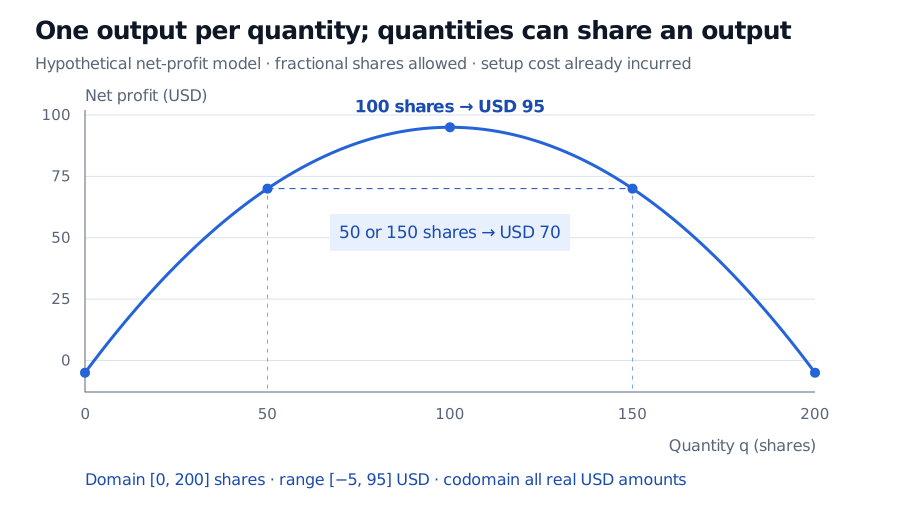
Hypothetical profit curve on 0 to 200 shares: 50 and 150 shares each produce USD 70; 100 shares produce USD 95; both endpoint quantities produce negative USD 5.
Original synthetic model. Each quantity determines one profit, although different quantities can give the same profit. The curve assumes fractional shares and an incurred setup cost.
On the stated interval, the squared term runs from 0 to 10,000, so profit runs from USD 95 down to negative USD 5 and takes every value in between. If only whole shares were allowed, the domain would instead be the integers from 0 to 200 and the range would be a finite set. The formula alone does not specify the whole function.
Single output does not mean unique input
The model gives Π(50)=Π(150)=70. This is a valid function: the rule forbids one input having two outputs, but permits two inputs sharing an output. Consequently, asking “which quantity produced USD 70?” has two answers. An inverse function requires an appropriate restriction before it can recover a unique quantity.
A graph records the pairs (x,f(x)). For a real-valued function of one real input, a vertical line meets that graph at most once. By contrast, the relation y2=x permits both y=2 and y=−2 at x=4, so it does not define a single-valued function of x without choosing a branch.
Functions need not arrive as formulas. A complete lookup table, a graph or a precise verbal rule can define one. Nor must an input or output be a single number: a multivariable pricing function can take a tuple of spot, strike, time, volatility and rates. Holding those other inputs fixed is what makes a graph against spot alone meaningful.
A function can represent an uncertain quantity
“Exactly one output per input” does not imply predictable markets. A random variable is itself a function: it assigns a numerical value to each possible outcome in a probability model, with a measurability condition that makes probabilities well defined. Before the outcome is known, its assigned value may be uncertain.
Likewise, the profit rule above gives a definite answer under its assumptions; uncertainty about future margins or costs requires additional inputs or a probabilistic model. Combining rules into stages leads to a composite function. The free full lesson Transformations, Compositions, and Building New Functions develops those operations, including how their domains fit together.
Sources
James Stewart, Single Variable Calculus: Early Transcendentals, 6th edition (2008), §1.1, “Four Ways to Represent a Function,” pp. 11–15.