A continuous-time process has a value at every time in an interval. Separate its clock, possible states and path continuity, then see what sampling an arrival count loses.
Continuous-time process
A continuous-time process is a stochastic process indexed by every time in an interval, such as {Xt:t≥0} or {Xt:0≤t≤T}. The model specifies a random quantity at each time, including times between recorded observations. This lets a quant model a default arriving between reporting dates or a price crossing a barrier between scheduled checks.
The word “continuous” describes the time index. It does not say that the values vary smoothly, that every real-valued state is possible, or that the process is observed continuously.
A Poisson process has continuous time, integer states and jumping paths. Brownian motion has continuous time, real states and continuous paths, although those paths are not differentiable almost surely. Both are continuous-time processes. Conversely, a sequence of daily real-valued returns has a discrete time index even though its modelled state space may be continuous.
At a fixed time, Xt is a random variable. Once an outcome is fixed, t↦Xt(ω) is one realised history. The clock alone specifies neither its distribution nor how different times depend on one another.
A count exists between the observations
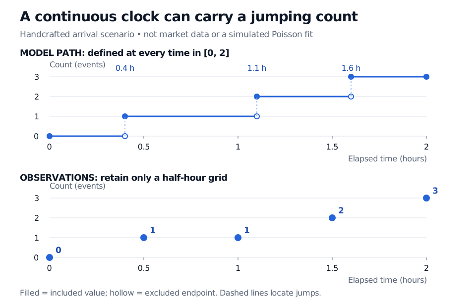
Consider a hypothetical system counting incoming execution requests over two hours. In one handcrafted scenario, requests arrive at 0.4, 1.1 and 1.6 hours after the start, with no other arrivals during the window. Let Nt count requests received at or beforet. The realised path is
The count is defined at every time in the window, stays constant between arrivals, and takes its new value immediately at each arrival. In particular, N0.5=1, N1=1, N1.5=2 and N2=3. No fractional requests are needed to fill in the intervening times.
An illustrative count jumps at 0.4, 1.1 and 1.6 hours. Half-hour observations at 0, 0.5, 1, 1.5 and 2 hours give counts 0, 1, 1, 2 and 3 while omitting the exact jump times.
Original handcrafted arrival scenario. Top: the full count path. Bottom: the half-hour observations. Filled endpoints belong to the path; hollow endpoints do not. The dashed vertical guides locate jumps, rather than fractional intermediate counts.
Now retain only a reading every 30 minutes. The sampled sequence Yk=Nk/2, for k=0,1,2,3,4, has discrete index k and values (0,1,1,2,3). It is a discrete-time observation of the continuous-time count. These observations locate arrivals within half-hour windows but cannot recover their exact timestamps. Drawing straight lines between the points would introduce fractional counts and an interpolation assumption absent from the counting model.
This single scenario illustrates the indexing distinction; it does not establish a Poisson law. Calling the requests Poisson would add specific distributional and independence assumptions. The membership lesson Defining the Poisson Process: Three Equivalent Constructions develops those assumptions from waiting times; its public page provides a preview.
Model clock, data clock, decision clock
A continuous-time price model can be fitted to daily observations and simulated on a finite grid. That calculation does not turn the underlying model into a discrete-time one; it evaluates or approximates selected parts of it. Equally, recording trades at irregular timestamps does not by itself specify a process between records.
For derivatives, the contract adds another clock: a continuously monitored barrier and a barrier checked only at scheduled times are different payoffs, even under the same continuous-time price model. A simulation grid can miss a crossing between grid points. Whether that is a numerical error or the intended contract convention depends on the monitoring rule.
Read “continuous time” as a commitment about when the model is defined. Check the state space, path assumptions, observation schedule and contractual monitoring separately.
Richard Durrett, Essentials of Stochastic Processes, third edition, Springer, 2016, §§2.2–2.2.1 — counts over continuous time and construction from arrival times.