A state space is the set of values that a model's state can take. In a credit model it might be rating labels; in a price model it might be positive real numbers. Choosing the state space determines what the model can represent—and which information a forecast may discard.
For a stochastic process, write
Here is the state space, is the time index set, and is the sample space of underlying outcomes. Formally, comes with a collection of measurable subsets so that statements about the state have well-defined probabilities. For a finite set, every subset can be used.
Three credit states, several different objects
Consider a hypothetical annual credit model with , where A and B are simplified rating buckets and D means default. These are stipulated model labels and probabilities, not agency data. Assume a time-homogeneous Markov model, start in A, and use this transition matrix:
| Current state / next year's state | A | B | D |
|---|---|---|---|
| A | 0.85 | 0.10 | 0.05 |
| B | 0.10 | 0.80 | 0.10 |
| D | 0 | 0 | 1 |
The state today is A. The state space remains all three labels. The time index is , with one year per step. One possible sample path over three observation times is : the entire sequence, rather than a single label.
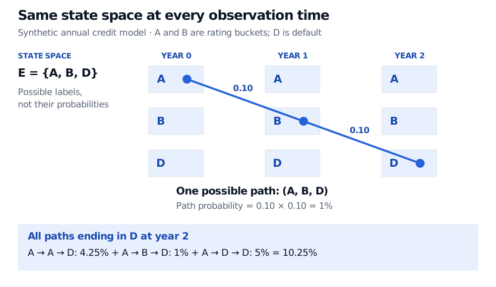
The blue connectors identify successive observations on one possible path; they do not describe a continuous rating between observations. The state labels alone do not determine the path probabilities.
Starting in A, the one-year default probability is 5%. At two years, add the contributions through each intermediate state:
Because D is an absorbing state, this 10.25% also means default by year 2. The final contribution includes borrowers already in D at year 1. The set has not changed between horizons; the probability distribution over it has.
State order is bookkeeping with consequences. The table uses order , and the initial row distribution is . If software stores states as , reorder both matrix axes and the initial distribution, now . The default probability stays 10.25%; merely relabelling column headings changes which economic event an entry describes.
Choosing what a state remembers
A daily return can have a real-valued state space even though observations arrive at discrete times. Conversely, an integer-valued trade count can evolve in continuous time. Time indexing and state values are separate choices; neither decides whether a path has jumps.
A richer state can be a vector: price alone takes values in , while a model tracking positive price and positive volatility uses . Those are different models of what must be retained. If default risk depends on time since downgrade, today's rating alone may lose predictive information. Including that duration enlarges the state. The Markov property is an additional assumption about the chosen state, not something guaranteed by naming its space.
For a prediction made today, the state must either be observed with today's information or inferred as a latent state; a future realised value cannot be smuggled into the forecasting input. A latent-state forecast carries uncertainty about the current state as well as about its future evolution.
Finally, the sample space describes underlying outcomes; the path space contains functions from time into . A fixed outcome produces the path . Some constructions take whole paths as the underlying outcomes, but a credit label by itself is neither an outcome history nor a path. An observed dataset is only a record of selected observations, not the model's full state space.
To develop the transition rules behind this example, SelfMadeQuant's Markov Chains — Transition Matrices and the Markov Property has a public preview; the full lesson requires membership. It also explains how retaining recent history can enlarge a state.
Sources
- Richard Durrett, Essentials of Stochastic Processes, third edition (Springer, 2016), §1.1: state specification, transition probabilities and state augmentation.
- Steven E. Shreve, Stochastic Calculus and Finance, notes prepared by Prasad Chalasani and Somesh Jha (Carnegie Mellon University, 25 July 1997), §1.1: outcomes, stock-price states and paths in a binomial model.
- Susan Holmes, Stanford University, Markov Chains — Stats 366 / Stats 166 course notes: finite states, row transition probabilities and two-step propagation.