A biased random walk is a random walk whose step distribution favours a direction. In the standard equal-size, two-direction model, independent steps go up with a fixed probability and down with probability , with . Its expected position moves through time, even though any particular path can move against that direction.
For a quant, this separates an assumed directional edge from the risk of a realised loss. A model with positive expected gains can still produce a losing run. Whether that assumed edge exists in market data is a separate estimation problem.
What the bias changes
Let be the size of each step, measured in the same units as the position. Starting from a fixed , define
with independent, identically distributed increments. The mean increment, or per-step drift, is . Thus
The expected value slopes upward for and downward for . At this becomes the symmetric random walk, with zero drift. At or , every step has the same sign and the variance is zero.
Here biased describes the step law. Bias of an estimator describes the difference between an estimator's expectation and its target parameter. A biased random walk need not be estimated with a biased estimator; the same word names different ideas.
Five chances to earn or lose one dollar
Suppose a hypothetical strategy starts at zero and takes exactly five independent trades. Each produces a gross gain of USD 1 with probability 60%, or a gross loss of USD 1 with probability 40%. These probabilities are stipulated, not fitted. There are initially no costs, funding constraints or early stopping.
Each trade has mean USD 0.20 and variance . After five trades,
The standard deviation is approximately USD 2.191. That is considerable dispersion around a one-dollar expected gain.
Let count the profitable trades. Then has a binomial distribution with and . The numerical result in dollars is . Earning at least USD 3 therefore requires four or five wins:
A gross loss requires at most two wins and has probability 31.744%. Zero is impossible after five equal unit steps: every endpoint is an odd number of dollars.
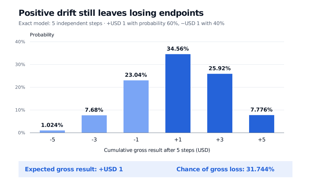
Original hypothetical model, exact probabilities rather than a simulated histogram. Lighter bars identify negative endpoints; the positive expected result does not exclude losses.
For the general count-to-position construction, Aldridge's university notes, §2.3, derive the exact endpoint law. Counting endpoints does not answer whether a path hit a loss limit earlier; imposing such a stopping rule changes the problem.
Put costs in the increments
Now change one assumption: charge USD 0.30 per trade, on every trade, regardless of outcome. Keep the same five-trade horizon and gross step law. Net increments become USD 0.70 and USD −1.30. The expected net increment is
Total fees are USD 1.50, so the expected net result is USD −0.50. A net profit now requires a gross result exceeding USD 1.50, hence at least USD 3 on this lattice. Its probability is the 33.696% calculated above. A win rate above 50% is insufficient by itself: payoff sizes and costs also determine the mean.
The raw biased walk is not a martingale under its natural history: its conditional expected next position differs from its current position by . Subtracting that accumulated drift gives , a martingale under the stipulated iid model. This mathematical centring does not remove the economic risk from an actual position.
To go beyond the endpoint calculation, SelfMadeQuant's Simple Random Walks — Symmetric and Asymmetric develops the model's step moments, Markov property and long-run behaviour. The full lesson requires membership; the linked page offers a public preview.
Sources
- Geoffrey Grimmett and David Stirzaker, Probability and Random Processes, 3rd edition, Oxford University Press, 2001, §3.9, pp. 71–72: independent two-direction steps, fixed step probabilities and the unconstrained walk.
- Matthew Aldridge, MATH2750, Section 2: Random walk, especially §2.3: the binomial count and exact endpoint support.