A regular payment stream valued by its timing: ordinary versus due annuities, present and future value, finite horizons and insurance-contract limits.
Annuity
An annuity is a stream of payments made at regular intervals. In elementary valuation, a level annuity pays the same amount each period. Its value depends on when the payments arrive, how long they continue and the discount rate used to compare them. Adding the payments alone does not tell you what the stream is worth today.
This cash-flow pattern appears in loan repayments, pension liabilities and fixed bond coupons. The word also names an insurance product. A mathematical payment schedule does not, by itself, specify an insurer, a guarantee or lifetime income.
Three payments, three different dates
Consider a certain payment of 100 currency units at each year-end for three years. Use a flat 5% annual effective interest rate, with annual compounding, and value the receipts immediately before the first year starts. Ignore fees, taxes and default. These are illustrative assumptions, not a product quote.
This is an ordinary annuity, also called an annuity-immediate: the first payment is one full period away. “Immediate” here does not mean a payment at time zero.
Calculations use unrounded values until the final display:
PV=1.05100+1.052100+1.053100≈272.32.
One way to interpret this amount is as a fund that finances the receipts. Start with the exact present value, earn 5% over the first year, and withdraw 100 at its end. Repeat the growth-and-withdrawal sequence twice more. The balance is exactly zero after the third withdrawal. Starting with the rounded 272.32 leaves a small rounding shortfall.
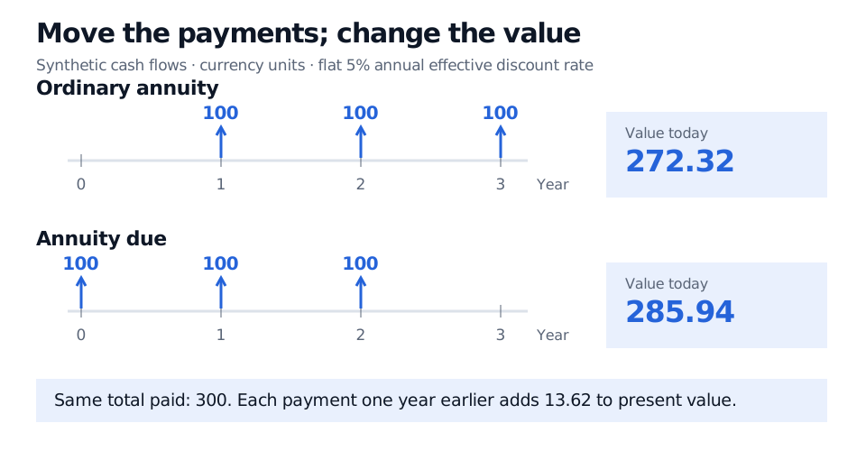
Now move every payment one year earlier: pay at times 0, 1 and 2. This is an annuity due. The payment today receives no discount; the others are discounted for one and two years. Its present value is 285.94, or 13.62 more than the ordinary annuity. At this positive rate, earlier receipts are more valuable.
Three receipts of 100 occur at years 1, 2 and 3 for an ordinary annuity, giving present value 272.32. Moving them to years 0, 1 and 2 gives an annuity due worth 285.94 at a flat 5% annual effective rate.
Same total payment, different timing. Original synthetic example; amounts are currency units and both values are measured at time zero.
The shortcut and its assumptions
For n equal payments of C, an ordinary annuity pays at periods 1,…,n. With a constant effective rate iper payment period,
PVordinary=Ck=1∑n(1+i)−k=Ci1−(1+i)−n,i=0.
The bracketed factor is the annuity factor: present value per unit of periodic payment. If i=0, use PV=nC directly; division by zero in the shortcut is not an economic problem. The finite sum remains meaningful for negative rates above −100% per period.
For the same number and size of payments shifted one period earlier,
PVdue=(1+i)PVordinary.
The factor 1+i follows from discounting each receipt for one fewer period. It is not an extra payment. At zero rates the two values coincide; at negative rates the earlier stream has the lower present value under this model.
A monthly stream needs a monthly effective rate. Do not automatically divide an effective annual rate by twelve: convert it to an equivalent monthly accumulation factor first. Also count payments, rather than substituting the number of years for n.
The future value of the ordinary stream, measured immediately after its final payment, is
FVn=Ci(1+i)n−1,i=0.
In our example this is 315.25 at year 3. The first 100 grows for two years, the second for one, and the last earns no interest before that valuation instant. Receiving 300 in total and accumulating 315.25 describe different quantities. That accumulation assumes every receipt can be reinvested at the stipulated 5%; actual future reinvestment rates need not match a rate used for valuation today.
For more on moving individual payments between dates, the Time Value of Money lesson explains accumulation and discount factors. It has a public preview; the full lesson requires membership.
Where the simple annuity stops
A flat rate is convenient, but a market yield curve can assign different discount factors to different dates. For fixed receipts at dates Tk, use
PV=Ck=1∑nD(0,Tk),
where D(0,Tk) is the appropriate discount factor for that receipt. Payment dates, currency and credit or collateral assumptions matter. Unequal accrual periods or changing payments require their actual amounts in the sum. For a fixed-coupon bond, the coupon stream may form an annuity, but the principal repayment must be valued separately.
A finite annuity ends after its stated payments. A perpetuity continues indefinitely; its shortcut cannot replace the finite annuity formula. A life-contingent annuity has a different uncertainty: payments may depend on survival, so its valuation needs mortality assumptions as well as financial discounting.
Insurance contracts sold as annuities can offer fixed or variable payments and different payout periods. Read the actual terms: a life-only payment, a guaranteed minimum payment period and a survivor benefit are different promises. Guarantees are contractual and depend on the issuer's ability to honour them; variable investment values can fall. The SEC's annuity overview and variable-annuity guide describe these distinctions for U.S. products.
Finally, level nominal payments do not guarantee level purchasing power. Inflation erodes what a fixed currency amount buys. A contract with escalating or inflation-linked payments needs its own cash-flow specification rather than the level-payment shortcut.
Sources
Frank J. Fabozzi and Francesco A. Fabozzi, Bond Markets, Analysis, and Strategies, 10th edition, MIT Press, 2021, Chapter 2, “Future Value of an Ordinary Annuity” and “Present Value of an Ordinary Annuity”; PDF pages 48 and 53–54 in the inspected local edition.