Calculate the future value of an initial balance and dated contributions, with a worked year-end versus year-beginning comparison and an original deposit-growth diagram.
Future value
Future value (FV) is the amount a present sum or a set of dated cash flows accumulates to at a specified future date, under stated growth assumptions. It answers “how much at the endpoint?” Where present value moves payments back to a valuation date, future value moves them forward.
The date is part of the answer. Money deposited today earns interest for longer than money deposited immediately before the endpoint. The rate convention is part of it too: 3.6% annual effective and 3.6% continuously compounded do not describe identical growth.
A research budget with three top-ups
A fictional quant research team sets aside money for a future data-licence payment. It starts with 7,200 USD today, then adds 1,800 USD at the end of each of the next three years. It wants the account balance at year three, immediately after the third top-up.
Assume the entire balance earns a fixed 3.6% annual-effective rate throughout. Interest remains in the account; there are no withdrawals, fees or taxes, and all deposits are made as planned. This is a stipulated calculation scenario, not a market forecast or a claim about an available deposit product.
For one deposit P that remains invested for n whole years,
FV=P(1+r)n,
where r=0.036 is the annual-effective rate. Compound interest means interest itself earns interest. The team's original 7,200 USD therefore becomes
7,200(1.036)3≈8,005.93 USD.
That is only one component of the final account balance. Each top-up needs its own remaining time.
The final contribution earns no interest
Deposit date
Amount deposited
Whole years until year 3
Value at year 3
Today, year 0
7,200 USD
3
8,005.93 USD
End of year 1
1,800 USD
2
1,931.93 USD
End of year 2
1,800 USD
1
1,864.80 USD
End of year 3
1,800 USD
0
1,800.00 USD
The last 1,800 USD is in the account at the measurement instant, but it has not had time to earn interest. Adding the accumulated components gives
The team contributed 12,600 USD, so 1,002.66 USD of the modeled final balance is interest. Treating all 12,600 USD as if it had been deposited today would overstate its time earning interest. Conversely, the increase from 7,200 to 13,602.66 is not all investment performance: much of it is additional money contributed.
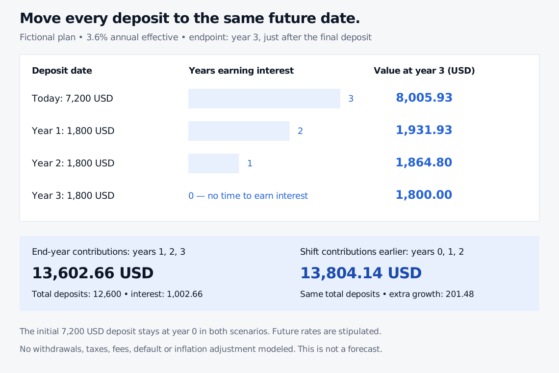
Deposits are moved to year three using the time each has actually been invested. The 7,200 USD initial deposit grows for three years; the 1,800 USD top-ups grow for two, one and zero years. Their future values sum to 13,602.66 USD. Shifting just the top-ups one year earlier produces 13,804.14 USD.
Original fictional calculation. The bars show years earning interest, not payment size. Both timing plans use the same total deposits and the same year-three endpoint.
Move the top-ups one year earlier
Now keep the original 7,200 USD deposit where it is, but make the three 1,800 USD top-ups at years 0, 1 and 2, rather than years 1, 2 and 3. At year three the balance becomes
The extra 201.48 USD comes from giving each top-up one additional year to grow. It does not come from contributing more money. Equal contributions at period ends are often called an ordinary annuity; moving them to the period beginnings gives an annuity due. These labels refer to payment timing here, rather than specifying an insurance product. OpenStax's annuity explanation develops the distinction.
Only the contribution stream is multiplied by one extra growth factor in this comparison. Multiplying the entire first balance by 1.036 would incorrectly move the initial 7,200 USD deposit as well. At zero interest, the timing change has no effect; with a negative rate, earlier contributions can leave a smaller final balance.
A common date makes the sum meaningful
For a constant annual-effective rate and deposits Ci at whole-year dates ti, the general calculation at year T is
FVT=i∑Ci(1+r)T−ti,ti≤T.
Deposits count positively in this account-balance calculation; withdrawals would reduce the balance. An investor's cash-flow ledger instead records deposits as outflows and a final withdrawal as an inflow. Keep that perspective consistent when calculating a return.
Under the same accumulation assumptions, discounting this final balance by (1+r)T recovers the present value of the dated deposits. This is the link to discount factors, not permission to add amounts at different dates without first moving them to a common date. OpenStax's time-value methods uses timelines to organise that comparison.
A future value is conditional on its inputs. Variable investment returns require the actual sequence of growth factors; an assumed constant rate does not remove risk. Nominal currency amounts do not automatically measure future purchasing power: inflation, taxes and fees need their own consistent treatment. Fractional periods also require the relevant accrual or compounding convention, rather than silently counting a partial year as a full one.
SelfMadeQuant's Time Value of Money lesson develops simple, periodic and continuous accumulation alongside discounting. Its public page is a preview; the full lesson requires membership. Continue with interest rate for quotations and day counts, or present value to reverse the direction of the calculation.
Sources
John C. Hull, Options, Futures, and Other Derivatives, Chapter 4, §§4.2–4.3: rate measurement and accumulation conventions.