A volatility term structure compares horizon-specific quotes. Learn why variance accumulates across time and why an ATM option curve is not a physical forecast.
Volatility term structure
The volatility term structure is the relationship between a volatility quote and its horizon, measured at one valuation time under a consistent set of conventions. For options, it usually means how implied volatility changes with time to expiry while holding a specified moneyness coordinate fixed. It lets a trader distinguish expensive near-term uncertainty from expensive longer-term uncertainty, rather than treating every option as having one volatility.
A term structure runs across maturities. A volatility smile runs across strikes at one maturity. The volatility surface combines both directions.
Say what each point measures
An ATM-forward option curve can be written as T↦σIV(0,T), where the first argument is log-forward-moneyness:
k=log(K/FT)=0.
Here K is strike, FT is the forward price for that expiry and T is a year fraction. Matching k does not generally mean matching the same cash strike across maturities.
Before comparing points, specify the underlying, valuation timestamp, expiry and settlement time, year-fraction convention, volatility annualisation, pricing convention and moneyness rule. A Black implied-volatility quote, a normal-volatility quote and the square root of a variance-swap strike measure different things. Mixing them can create a curve with no coherent interpretation.
A longer-horizon volatility quote averages uncertainty over its whole horizon. It does not describe only the period after the shorter expiry. The clean additive example uses variance swaps, rather than assuming that an ATM option quote is a variance-swap strike.
Consider synthetic contracts on the same underlying, starting now. Stipulate continuously measured integrated variance A(0,T)=∫0Tvudu, zero deterministic interest rates, and identical variance definitions and year clocks. Under one common risk-neutral measure, a fair annualised variance strike is
Kvar(T)=TEQ[A(0,T)].
Write its volatility-style quote as σvar(T)=Kvar(T). This is the square root of a variance strike, not the fair strike of a volatility swap. The accumulated expected variance is
W(T)=Tσvar(T)2.
The following quotes are stipulated teaching inputs, not observed market prices. All times are exact year fractions; volatility percentages are annualised and squared using decimal returns.
Horizon from now
Volatility-style variance-swap quote
Annualised variance strike
Accumulated expected variance
T1=0.25 year
20%
0.0400
0.0100
T2=1.00 year
25%
0.0625
0.0625
Because the integrated variance of adjacent intervals adds on every path, its expectation adds too:
EQ[A(T1,T2)]=W(T2)−W(T1).
Thus the annualised expected variance for the remaining 0.75 year is
The interval's root expected variance exceeds both whole-horizon quotes. Its higher level is needed to lift the full-year average above the first quarter's level. Subtracting 25%−20% would give a volatility-level difference of five percentage points, which does not measure the interval's volatility.
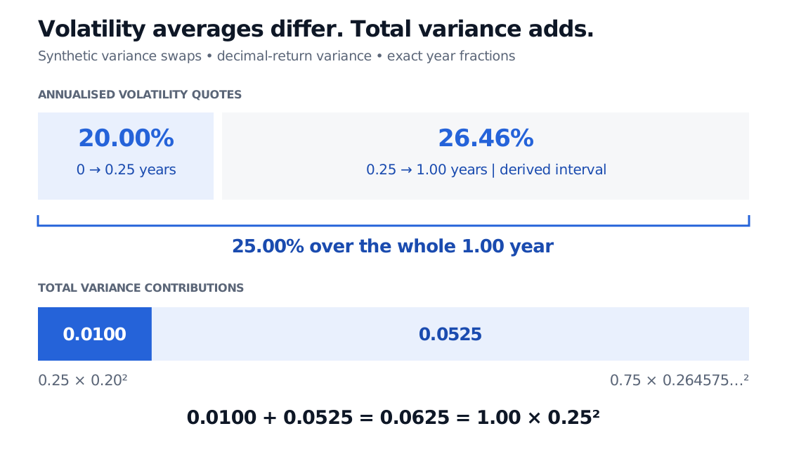
Synthetic variance-swap quotes are 20% for 0–0.25 years and 25% for 0–1 year. The 0.25–1-year interval has 26.46% root expected annualised variance. Accumulated expected variance adds as 0.0100 plus 0.0525 equals 0.0625.
The upper blocks show horizon-average volatility quotes; their widths represent time. The lower blocks show expected integrated-variance contributions; their widths represent variance. Synthetic continuous-variance contracts, zero interest rates and one common pricing measure.
This is a pricing expectation. It does not say that realised future volatility will be 26.46%, or that the corresponding expectation under the physical probability measure is the same. The volatility risk premium is one reason pricing and forecasting quantities differ. Actual contracts also require attention to sampling, caps, annualisation and payment dates before combining exposures.
What an option curve can establish
For Black implied volatility at fixed k, total implied variance is w(k,T)=TσIV(k,T)2. Taking its maturity difference is useful for a model or interpolation diagnostic. It is not automatically the expected integrated variance above, a variance-swap replication, or the implied volatility of an actual forward-starting option. In a model with deterministic time-dependent variance, the averaging relation has a direct interpretation; general stochastic-volatility models require more information.
A falling annualised volatility curve can coexist with increasing total variance: the longer horizon can accumulate more uncertainty at a lower average rate. Consequently, a downward slope alone does not demonstrate arbitrage. Nor does an upward slope prove that investors forecast rising realised volatility.
For European option surfaces under the appropriate proportional-dividend and forward-normalisation assumptions, the calendar condition is non-decreasing w(k,T) at every fixed k. Checking only an ATM curve cannot certify a whole surface: other moneyness levels, within-expiry option-price convexity, boundaries and interpolation still matter. Gatheral and Jacquier's analysis separates the calendar and butterfly conditions explicitly.
Sources
Jim Gatheral, The Volatility Surface: A Practitioner's Guide, Wiley, 2006, Chapter 3, pp. 27–29 (implied-variance weighting and the deterministic-volatility special case); Chapter 11, pp. 137–139 and 143–144 (variance swaps, ATM implied volatility and the volatility-swap distinction).
Jim Gatheral and Antoine Jacquier, Arbitrage-free SVI volatility surfaces, §2, especially Lemma 2.1: fixed-forward-moneyness calendar conditions and the separate butterfly requirement.
Jim Gatheral and Martin Keller-Ressel, Affine forward variance models, §2.1: forward variance as a conditional expectation of future instantaneous variance.