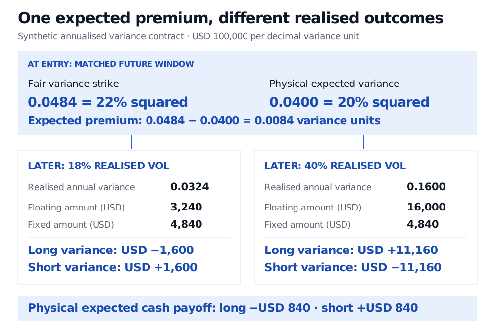
Separate the variance risk premium from realised trading profit, with explicit physical and pricing expectations, quote units and a synthetic cash-settlement ledger.
Volatility risk premium
The volatility risk premium (VRP) is the compensation associated with bearing uncertainty about future volatility. In a common, measurable formulation, it is the gap between the price of future variance and its expected realised level under real-world probabilities. A positive gap can give a seller of variance a positive expected payoff while leaving that seller exposed to a large loss when volatility surges.
The name needs a convention. This page uses risk-neutral expected variance minus physical expected variance, often called the variance risk premium. Other sources reverse the sign or work in volatility rather than variance units; compare their definitions before comparing their numbers.
Price and forecast answer different questions
Let RVt,T be realised variance, annualised according to a specified contract, over the future window from t to T. Write Kvar,t,T for the fair fixed variance strike of a zero-value-at-entry variance swap. Under the convention here,
VRPt,T=Kvar,t,T−EtP[RVt,T].
The physical measure P describes real-world probabilities. Its conditional expectation is a forecast of the future contract measurement, using information available at entry. A past historical-volatility estimate can be a forecasting input; it does not automatically equal that future expectation.
With deterministic discounting and the usual frictionless risk-neutral valuation assumptions, the fair strike satisfies
Kvar,t,T=EtQ[RVt,T],
so the premium is a Q-minus-P expectation gap for the same future quantity. The risk-neutral measure Q incorporates how states are priced; it is not simply a more accurate real-world forecast. Londono and Xu, §3.1, explicitly define their variance premium using these two expectations.
The discounting assumption matters. With stochastic interest rates, let Dt,T be the money-market discount factor and Q the corresponding risk-neutral measure. Zero entry value instead gives
Kvar,t,T=EtQ[Dt,T]EtQ[Dt,TRVt,T].
This is also an expectation under the corresponding T-forward measure. It need not equal the unweighted money-market-measure expectation. Credit, collateral and trading-cost adjustments also require their own treatment. Demeterfi, Derman, Kamal and Zou, pp. 15–17, develop the risk-neutral valuation argument for variance swaps.
For the reasoning behind pricing with Q rather than a physical forecast, the owned lesson Market Model and Risk-Neutral Valuation derives the distinction from replication and explains incomplete markets. Its preview is public; the full lesson requires membership.
A premium known only through an estimate
Consider a synthetic contract whose strike and forecast refer to the same future observation window, return definition and annualisation rule. Use decimal-return variance units. Stipulate deterministic zero discounting, no initial payment, fees, funding, margin cash flows, tax or default.
Quantity at entry
Annual variance, decimal-return basis
Fair variance strike, quoted as 22% volatility squared
0.222=0.0484
Model's physical expected realised variance
0.202=0.0400
VRP, using strike minus physical expectation
0.0084
The 20% is the square root of expected variance, not necessarily expected realised volatility. The physical expectation is a stipulated model forecast, not something directly revealed by the swap quote.
On a squared-percentage-point scale, multiply every variance by 10,000: the entries become 484, 400 and 84. The premium is not two volatility percentage points. The difference 22%−20%=2 percentage points belongs to a different scale, and even there the 20% is a root-mean-square quantity.
Take a variance notional N=100,000USD per one decimal annual variance unit. At maturity, the long receives floating variance and pays the fixed strike:
Long payoff=N(RVt,T−Kvar,t,T).
The short receives the opposite amount. Equivalently, use USD 10 per squared-percentage-point variance unit; changing the variance scale without changing the notional would change the exposure by a factor of 10,000.
Realised annual volatility
Realised variance
Long's floating amount, USD
Long's fixed amount paid, USD
Long's net payoff, USD
Short's net payoff, USD
18%
0.0324
3,240
4,840
−1,600
+1,600
22%
0.0484
4,840
4,840
0
0
40%
0.1600
16,000
4,840
+11,160
−11,160
The floating and fixed columns decompose a single net cash settlement. There is no exchange of the USD 100,000 notional principal. With the stipulated zero entry payment and excluded costs, net payoff also equals the contract's cash profit.
At entry, the model-implied physical expected long payoff is instead
100,000(0.0400−0.0484)=−840 USD.
The short's expected payoff is +USD 840. Neither equals the eventual payoff in every outcome. A positive premium is compensation for a risk exposure, not a certain profit or a percentage return on capital; a return calculation also needs a defined capital or margin denominator.
Synthetic variance contract: strike 0.0484 minus physical expected variance 0.0400 gives an expected premium of 0.0084. At 18% realised volatility, long variance loses USD 1,600; at 40%, it gains USD 11,160. The short has opposite payoffs. Physical expected long payoff is minus USD 840.
Original synthetic ledger. All variance values use decimal returns and annualisation; the cash notional is USD 100,000 per variance unit. The entry premium estimate and the two later settlement scenarios are different objects.
Three distinctions that prevent false signals
An estimate is not a realised spread. At expiry, strike minus realised variance is an ex-post outcome. At entry, strike minus expected future variance is an ex-ante premium estimate. Subtracting last month's realised variance from next month's implied variance creates a proxy whose usefulness depends on its forecasting assumptions. Bollerslev and Zhou, §2.1, distinguish their lagged-realised proxy from both a matched-window ex-post spread and a conditional-expectation premium.
A variance quote is not a single option's implied volatility. The 22% above means Kvar. A single option's implied volatility comes from inverting a particular pricing model at a particular strike and maturity. A variance strike reflects a different payoff; under continuous-path idealisations it can be related to an entire strip of options. Skew, limited strikes, jumps and sampling conventions matter. Gatheral's The Volatility Surface, Chapter 11, treats this distinction.
Expected volatility is not the square root of expected variance. Since the square root is concave, Jensen's inequality gives, under either specified measure M,
EtM[RVt,T]≤EtM[RVt,T].
Equality requires conditionally constant realised variance. A volatility-swap premium therefore cannot generally be obtained by taking square roots of the two variance expectations and subtracting them. The same horizon, measure, units and settlement definition must accompany any reported VRP number.
Kresimir Demeterfi, Emanuel Derman, Michael Kamal and Joseph Zou, More Than You Ever Wanted To Know About Volatility Swaps (March 1999), pp. 3–4, 15–17 and 33–34: swap payoffs, fair strikes and variance-to-volatility convexity.
Jim Gatheral, The Volatility Surface: A Practitioner's Guide, first edition, Wiley (2006), Chapter 11, especially pp. 137–139: variance contracts and their relation to option-implied volatility. Local edition and cited sections checked.