A transition probability conditions a future state on a starting state. See why tomorrow’s conditional probability differs from a marginal forecast and a two-day forecast.
Transition probability
A transition probability is the conditional probability of a future state given a specified starting state. In a credit-migration or market-regime model, it answers “where might the system go from here, over this horizon?” The starting information and time interval are part of the quantity, not optional labels.
For a discrete-state process observed each day, a one-day transition probability is
pij(n)=P(Xn+1=j∣Xn=i).
Here i is today's state and j tomorrow's. The probabilities across all possible destinations sum to one for each starting state. With the row convention, these probabilities form row i of a transition matrix.
Writing this conditional probability does not itself impose the Markov property. That additional assumption says earlier history supplies no further predictive information once the current state is known. Time-homogeneity adds another restriction: the transition probabilities do not depend on the starting day n. A model can be Markov while its transition probabilities change over time.
Four questions, four probabilities
Consider a hypothetical time-homogeneous daily Markov chain with two states, Calm and Stress. From Calm, tomorrow is Stress with probability 0.20; from Stress, tomorrow remains Stress with probability 0.70. The complementary probabilities of Calm are 0.80 and 0.30. These are stipulated teaching assumptions, not a fit to market data.
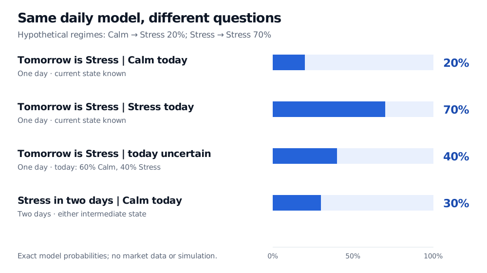
If today is known to be Calm, tomorrow's Stress probability is 20%. If today is known to be Stress, it is 70%. These are different conditional forecasts, each using its own starting state.
Suppose instead the information used for a forecast assigns today probabilities 60% Calm and 40% Stress. The marginal distribution of tomorrow mixes both possible starting states:
P(Xn+1=S)=0.60(0.20)+0.40(0.70)=0.40.
This 40% forecast is neither entry by itself. It uses uncertainty about today's state as well as the transition rule.
Now change the horizon: starting definitely in Calm, what is the probability of Stress in two days? There are two disjoint routes to that endpoint:
P(Xn+2=S∣Xn=C)=0.80(0.20)+0.20(0.70)=0.30.
The route through Calm contributes 0.16; the route through Stress contributes 0.14. Squaring 0.20 would miss the intermediate-state possibilities. Summing over them is the idea behind the Chapman–Kolmogorov equations.
Four exact Stress probabilities in a hypothetical daily model: 20% tomorrow given Calm today; 70% tomorrow given Stress today; 40% tomorrow when today is 60% Calm and 40% Stress; 30% in two days given Calm today.
The conditioning information and forecast horizon identify the probability. Bars share a 0–100% probability scale; these are stipulated model results, not estimated market frequencies.
The two-day endpoint probability does not mean “Stress occurs at any time during the next two days.” A path can enter Stress on day 1 and return to Calm on day 2. Barrier and default questions need their event defined carefully; an absorbing default state is a special case in which arrival persists.
A model input can be an estimate
A daily transition probability is dimensionless, but daily specifies its horizon. Reusing it as an annual probability changes the model. Nor is it a continuous-time transition rate, which has units of inverse time.
When states are observed, a common estimate divides the number of observed i-to-j transitions by the total observed departures from i, including self-transitions. A row with no observed departures cannot be estimated by that ratio. Such frequencies are estimates with sampling uncertainty; they do not establish stable probabilities or prove the Markov assumption. State definitions, observation frequency, regime changes and hidden-state uncertainty can all change the forecast.
To develop the state-based model further, Markov Chains — Transition Matrices and the Markov Property connects transition diagrams with credit-rating examples. The full lesson requires membership; the linked public page provides a preview.
Sources
Richard Durrett, Essentials of Stochastic Processes, third edition (2016), §§1.1–1.2: conditional transition rules, time-homogeneity and multistep transitions.
Susan Holmes, Stanford University, Stats 366 / Stats 166: Markov Chains: conditional-state interpretation, matrix powers and averaging over starting states.