Understand the spacing of a computational time grid, audit a fixed-horizon Euler calculation, and separate numerical updates from market observations and contract monitoring.
Time step
A time step is the length of time between two successive points on a computational time grid. It determines how far a simulation or numerical solver advances before updating its state. In option pricing, that choice can change the computed price, the work required and whether the chosen scheme behaves reliably.
For a grid 0=t0<t1<⋯<tN=T, the individual steps are hn=tn+1−tn. On a uniform grid they are all equal:
h=Δt=NT,tn=nh.
There are N intervals but N+1 grid points, including the initial and final points. The horizon T is the total duration; h is the spacing within it. Reducing h while keeping T fixed increases the number of updates.
One year, three grids
Consider a deliberately simple deterministic account model, with no cash flows:
dtdV=aV,a=0.10per year,V(0)=100USD.
This stipulates a continuous growth rate, not a forecast of market returns. Its exact one-year value is V(1)=100e0.1≈110.51709180756 USD.
The forward Euler method freezes the growth calculation at the start of each interval:
Vn+1=Vn+ahVn=(1+ah)Vn.
With h measured in years, ah is dimensionless. Using a rate quoted per year with an unconverted step measured in days would change the model calculation.
Intervals N
Step h (years)
Euler value at one year (USD)
Absolute error (USD, rounded)
1
1
110
0.517092
2
0.5
110.25
0.267092
4
0.25
110.3812890625
0.135803
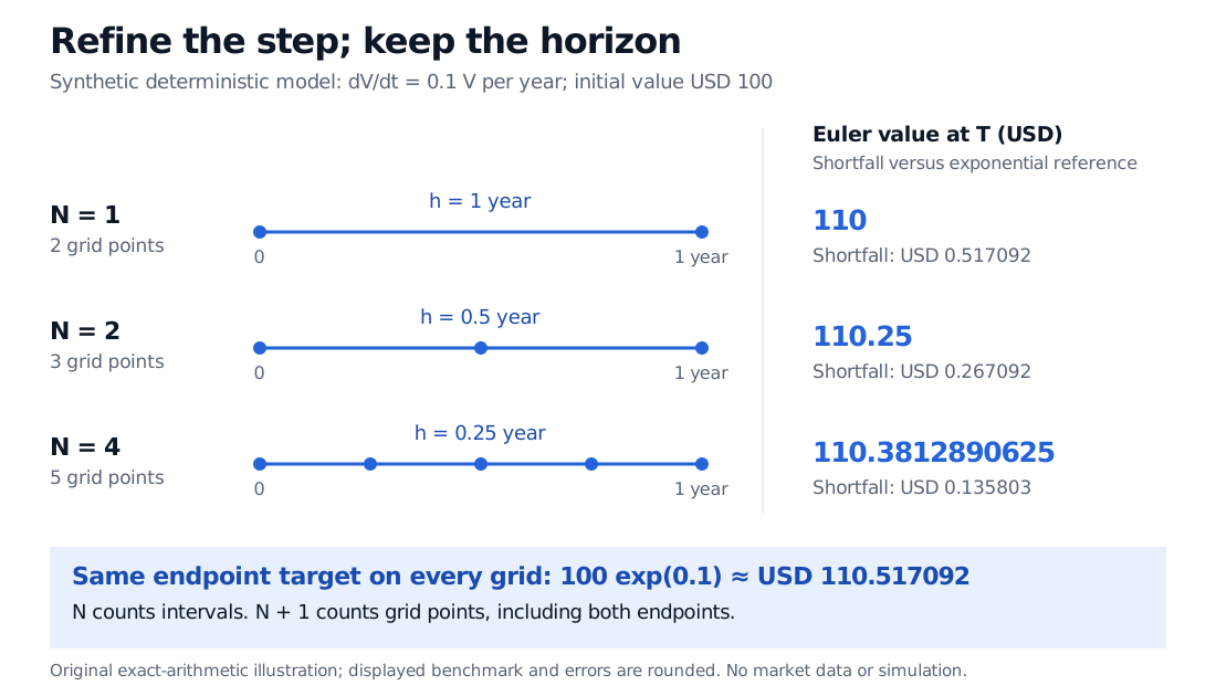
For two intervals the account moves from USD 100 to USD 105, then to USD 110.25. The second update earns growth on the already updated balance. More frequent updates bring this particular approximation closer to the stipulated continuous model.
Three grids cover the same one-year horizon. N equals 1, 2 and 4 uses 2, 3 and 5 points with steps 1, 0.5 and 0.25 years. Euler values are USD 110, USD 110.25 and USD 110.3812890625; rounded shortfalls are USD 0.517092, USD 0.267092 and USD 0.135803.
Original deterministic example. The horizon and model stay fixed as the step shrinks. The benchmark and error labels are rounded; no market data or random paths are used.
The discrepancy is discretisation error from the numerical update. It is not uncertainty about the model's answer. Nor does choosing a time step require an approximation: replacing Euler's factor by the exact factor eah gives
VN=100(eah)N=100eaT
on every uniform grid in exact arithmetic. The update rule and the time step must be considered together.
Three clocks that need not coincide
Computational grid: the dates at which an algorithm updates its state. A nonuniform grid can use shorter intervals near an event, and an adaptive solver can select intervals as it runs.
Observation interval: the spacing of recorded market data. A finer computational grid does not create additional observations or eliminate uncertainty in estimated inputs.
Contractual monitoring dates: the dates on which a barrier or another contract condition is checked. Changing a discretely monitored contract to more frequent monitoring changes its payoff rule; refining an internal calculation should preserve that rule.
For geometric Brownian motion, exact transitions can remove the time-integration error at sampled dates. They do not reveal every movement between those dates. A continuously monitored barrier can be crossed between two sampled values even if both are below it; appropriate crossing methods, such as Brownian bridge calculations, address a different problem from exact endpoint sampling.
Choosing a step is an error-and-cost decision
Compare several grids at the same horizon and inspect the quantity that matters: a terminal value, an option price or a Greek. Convergence concerns the limiting behaviour as the mesh is refined; a short table of improving values is evidence for that example, not a general guarantee.
The scheme's order of accuracy describes error scaling under stated assumptions. Its numerical stability concerns how errors propagate. In the growing account example, a factor above one is expected: increasing balances alone do not demonstrate numerical instability.
Smaller steps require more updates and can expose rounding or other error sources. In a PDE solver the allowed time step can also depend on the spatial grid and the method. SelfMadeQuant's Finite Difference Methods lesson develops these coupled grids and compares explicit, implicit and Crank–Nicolson updates; the full lesson requires membership, with a public preview available.
Sources
Tobin A. Driscoll and Richard J. Braun, Fundamentals of Numerical Computation, §6.2, Euler's method: uniform time grids, explicit updates and fixed-horizon convergence.
Rüdiger U. Seydel, Tools for Computational Finance, 6th edition, Springer, 2017, §1.7.1, Algorithm 1.11, pp.42–43; Chapter 3, pp.125–127; and §3.4, pp.139–140: time-grid conventions, deterministic and stochastic discretisation, and within-step bridge questions.