A Brownian bridge pins both endpoints while leaving a random interior. Derive its conditional mean and covariance, then see why endpoint knowledge changes simulation.
Brownian bridge
A Brownian bridge is a continuous Gaussian process describing Brownian motion between a known starting value and a specified value at a future time. Both endpoints are pinned; the route between them remains random. That distinction matters when simulating a path-dependent payoff: observing the price at two dates does not reveal what happened between those dates.
The standard bridge starts and ends at zero over [0,1]. It is not an ordinary Brownian motion that happens to have a small final value. Fixing the endpoint changes the distribution of the whole path.
Remove the endpoint, keep the fluctuations
For standard Brownian motion Wt, define
Bt=Wt−tW1,0≤t≤1.
The subtraction removes the straight line joining zero to the realised endpoint. Consequently B0=B1=0, and the mean is zero at every time. Because this is a linear transformation of jointly normal variables, B is a Gaussian process. Its mean and covariance therefore determine every finite collection of values.
Using Cov(Ws,Wt)=min(s,t) gives
Cov(Bs,Bt)=min(s,t)−ts−st+st=min(s,t)−st.
In particular,
Var(Bt)=t(1−t).
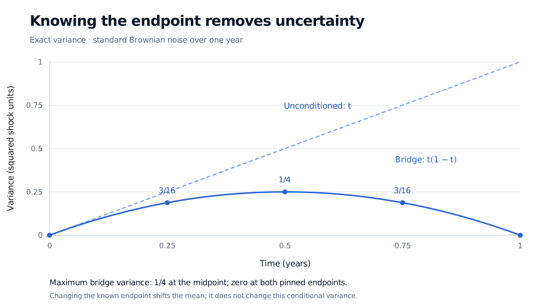
Uncertainty grows away from the known starting point, then contracts as the known destination approaches. Its maximum is 1/4 at the midpoint. At quarter, half and three-quarter time, the variances are 3/16, 1/4 and 3/16 respectively.
Exact bridge variance is t(1 minus t), reaching 1/4 at half a year and 3/16 at quarter and three-quarter time; unconditioned Brownian variance grows as t.
Original exact variance curves over one year. Changing the known endpoint shifts the conditional mean but leaves this conditional variance unchanged.
The bridge values are dependent. For example, Cov(B1/4,B3/4)=1/16. Its increments also lose Brownian motion's independence: the final increment must undo whatever displacement remains before the fixed endpoint.
A known endpoint is a conditional distribution
Suppose time is measured in years and W1=0.4. In standardized shock units, the path conditional on that endpoint has the same distribution as
Xt=0.4t+Bt.
The key is that B is independent of W1: its covariance with that endpoint is zero, and the relevant variables are jointly Gaussian. This decomposition separates the information supplied by the endpoint from the remaining uncertainty. Pitman's Berkeley notes, pp. 2–3, explain this conditional interpretation.
At the midpoint,
W0.5∣W1=0.4∼N(0.2,0.25).
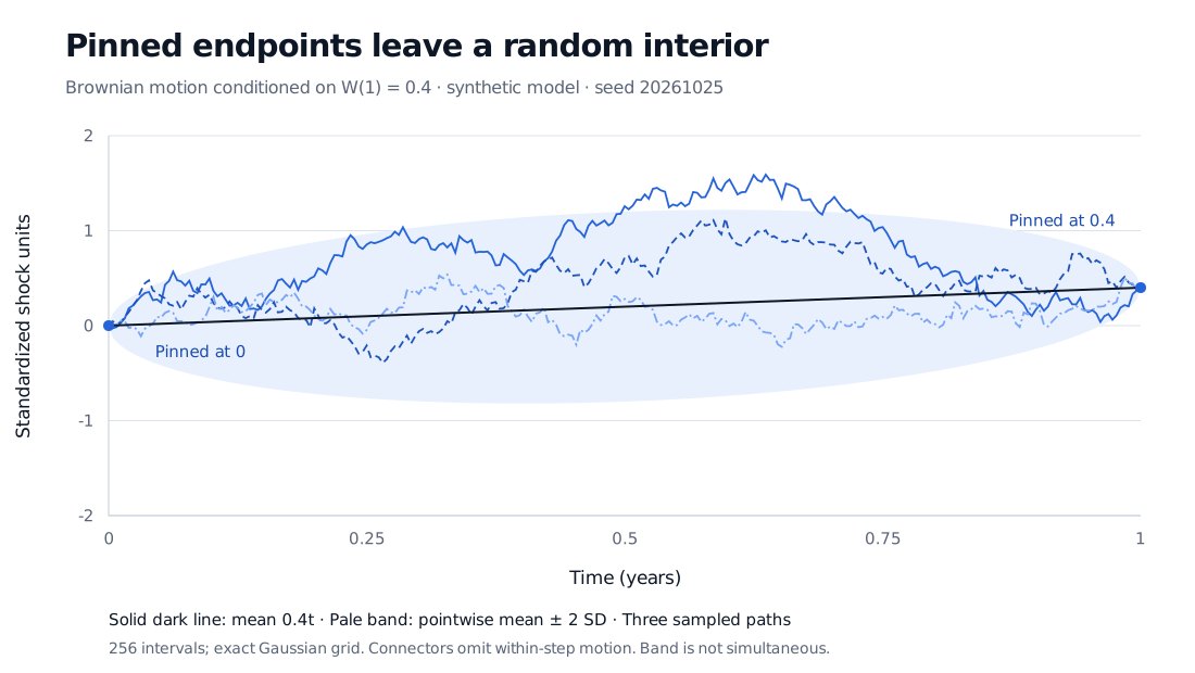
Here the second normal parameter is variance. The conditional mean is 0.2, while the standard deviation is 0.5. A two-standard-deviation interval is therefore [−0.8,1.2], containing about 95.45% of the midpoint distribution. Knowing the final value does not force the halfway value to lie near the straight line.
Three seeded conditional Brownian paths join 0 to 0.4 over one year. The mean is 0.4t; the pointwise two-standard-deviation band has midpoint interval minus 0.8 to 1.2.
Original synthetic Gaussian paths, seed 20261025, sampled on 256 equal intervals. The pale band is mean ± 2 standard deviations at each fixed interior time; its 95.45% coverage is pointwise, not a probability that the entire path stays inside. Straight connectors omit movement between samples.
There is a technical subtlety: P(W1=0.4)=0. The conditional law uses the regular conditional Gaussian distribution, or an appropriate limit of conditioning on a shrinking interval around 0.4; it is not division by the probability of a single endpoint. Simulation constructs this conditional law directly, rather than repeatedly drawing unconstrained paths until one hits exactly 0.4.
Different endpoints, horizons and scales
A bridge from a to b over [0,T], with T>0 and constant diffusion scale σ>0, can be represented as
If time is measured in years and state in points, σ has units of points per square-root year. The endpoints determine the affine mean; the horizon and diffusion scale determine the remaining dispersion. These formulas describe constant-diffusion Brownian conditioning, not an arbitrary financial model conditioned on its terminal price.
The construction uses WT, so for an interior time it looks into the future of the original Brownian motion. It is therefore not adapted to that original motion's past filtration. The bridge has its own natural filtration; distributional equivalence does not make these two information flows interchangeable.
Fill the middle after the ends. A simulator may sample a Brownian terminal value first, then sample the midpoint conditionally, and repeat inside each interval. With the correct conditional Gaussian distributions, this gives the same Brownian grid law as sampling independent increments from left to right. It changes the order in which randomness enters the path. That can help some quasi-Monte Carlo integrations, but it does not guarantee an efficiency gain for every payoff. Glasserman's §3.1 derives this construction.
Account for unobserved crossings. For a continuously monitored barrier, endpoints on the safe side do not establish that the entire intervening path was safe. Brownian bridge laws support conditional crossing calculations under suitable models. A bridge in a constant-volatility log-price model differs from a bridge in the price level itself; assumptions and monitoring conventions must match the contract. Plotting more straight segments is not a crossing calculation.
Practice: give the endpoint back
Let Bt be a standard bridge and let Z∼N(0,1) be independent of the whole bridge. Does Yt=Bt+tZ, for 0≤t≤1, have the law of standard Brownian motion?
Answer. Yes. It is a continuous Gaussian process starting at zero, with mean zero and
Cov(Ys,Yt)=min(s,t)−st+st=min(s,t).
These are the Brownian mean and covariance, so the Gaussian finite-dimensional laws agree. The terminal value is now Y1=Z rather than a fixed number. Choosing Z independently is essential; matching the endpoint's marginal distribution alone does not ensure the correct joint path law.
Sources
Ioannis Karatzas and Steven E. Shreve, Brownian Motion and Stochastic Calculus, first edition (Springer, 1988), Chapter 5 §6B, pp. 359–360: Gaussian bridge mean, covariance, conditional law and endpoint-subtraction representation.
Paul Glasserman, Monte Carlo Methods in Financial Engineering (Springer, 2004), §3.1, pp. 83–86: conditional Gaussian interpolation and Brownian bridge path construction.
Jim Pitman, Stat 150: Lecture 28, Brownian Bridge, University of California, Berkeley, Spring 2009, pp. 2–3: independence of the residual bridge and endpoint, and conditioning on a specified terminal value.
Kyle Siegrist, The Brownian Bridge, Random Services: bridge constructions and recovery of Brownian motion by adding an independent normal endpoint.