Range restriction correction: Definition & Examples

Range restriction correction estimates the correlation in a broader population from a correlation observed over a selected, narrower range of values. Its best-known direct-selection formula combines the selected correlation with external information about the predictor's spread. For a quant evaluating a signal within a filtered asset universe, it explains why a smaller correlation can reflect a narrower score range even when the underlying response to the score is unchanged.

The correction answers a population-comparison question. It does not automatically make a signal more useful in the actual universe being traded: that universe may genuinely offer less variation to exploit.

The slope can survive while correlation shrinks

Suppose a fictional score

X

and subsequent return

Y

, measured in percentage points, obey

Y=0.4X+\varepsilon, \qquad \mathbb{E}[\varepsilon\mid X]=0, \qquad \text{Var}(\varepsilon\mid X)=0.84.

These are stipulated model quantities, not estimates from market data. Selection retains observations solely according to

X

, leaving the conditional distribution of the error unchanged. The linear regression slope is therefore still

0.4

percentage points per score unit after selection.

Let the full universe have $\text{Var}(X)=4$ and the selected band have $\text{Var}(X\mid S=1)=1$ , where $S=1$ means retained. One exact construction makes $X$ equally likely to be $-\sqrt7,-1,1,\sqrt7$ , with independent error equally likely to be $-\sqrt{0.84}$ or $\sqrt{0.84}$ . Keeping only $|X|\leq1$ retains four of the eight equally likely states. Both populations have zero means.

The variance of

Y

is the score-driven variance plus the error variance. The resulting population moments are:

Quantity	Selected band	Full universe
Variance of $X$ , score units squared	$1$	$4$
Score-driven variance of $Y$ , percentage points squared	$0.16$	$0.64$
Error variance, percentage points squared	$0.84$	$0.84$
Total variance of $Y$ , percentage points squared	$1$	$1.48$
Correlation	$0.4000$	$0.6576$
Regression slope, percentage points per score unit	$0.4$	$0.4$

For example, full-universe covariance is $0.4\times4=1.6$ , so its correlation is

\rho_U=\frac{1.6}{2\sqrt{1.48}} =\frac{0.8}{\sqrt{1.48}} \approx0.65759595.

The selected correlation is $0.4/(1\times1)=0.4$ . Holding error dispersion fixed, narrowing the score range reduces the signal's contribution relative to the noise. Neither the slope nor the conditional error law had to deteriorate.

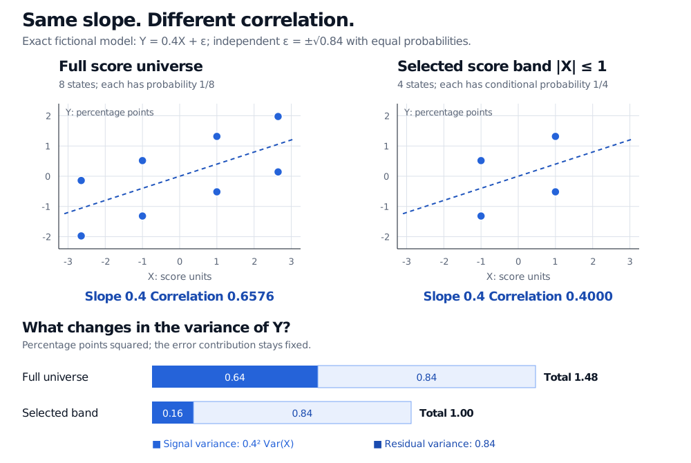
An exact fictional eight-state model retains four states with absolute score at most one. The slope remains 0.4; correlation falls from 0.6576 to 0.4000. Score-driven return variance falls from 0.64 to 0.16 percentage points squared, while residual variance stays 0.84.

Exact fictional distribution, not market observations. Both plots use the same axes; dashed lines show the common conditional mean. The variance bars separate the changing score contribution from the fixed error contribution.

Thorndike's direct-selection formula

For this case, define

\rho_R=\operatorname{Corr}(X,Y\mid S=1)

and the standard deviation ratio

u=\frac{\sigma_{X,U}}{\sigma_{X,R}}.

Here unrestricted goes in the numerator:

u=2

. Under a common linear conditional mean and constant conditional error variance, with selection depending only on

X

\rho_U=\frac{u\rho_R}{\sqrt{1+\rho_R^2(u^2-1)}}.

This is the direct range-restriction correction commonly called Thorndike Case II; some sources define the spread ratio as the reciprocal. Osnabrück University's MethodsLab gives both conventions explicitly.

For the worked model,

\rho_U=\frac{2(0.4)}{\sqrt{1+0.4^2(2^2-1)}} =\frac{0.8}{\sqrt{1.48}} \approx0.6576.

Simply multiplying $0.4$ by $2$ would incorrectly give $0.8$ : the denominator adjusts for the fact that the full-universe variance of $Y$ also changes.

To see the formula's origin, write $Y=a+bX+\varepsilon$ and let the common error variance be $\tau^2$ . In either population,

\rho=\frac{b\sigma_X}{\sqrt{b^2\sigma_X^2+\tau^2}}.

Substituting $\sigma_{X,U}=u\sigma_{X,R}$ and eliminating $b$ and $\tau$ gives the correction. Finite second moments and positive predictor and response variances are required. Normality is unnecessary for this moment argument; the preserved linear mean and homoskedasticity do the work.

With estimated inputs, the result is a corrected estimate, not an exact population recovery. Sampling error in the selected correlation and uncertainty in the external spread both matter. In the exact formula,

u=1

makes no adjustment, and

u>1

increases the magnitude while preserving the sign. A zero restricted correlation stays zero under these assumptions.

First establish what selected the sample

The full-universe spread must describe the intended target universe, on the same score definition and scale. It might come from scores recorded for all eligible assets even though outcomes are analysed only for a subset. It cannot generally be recovered from the selected sample alone. A historical spread from a different market regime or a differently normalised score is not automatically suitable.

This direct formula is not a general cure for selection bias:

If inclusion uses realised $Y$ , another signal, or a composite of scores, the direct-selection assumptions need separate justification. Knowing only the two spreads of $X$ is generally insufficient.
If the response bends outside the observed band, or error variance changes with the score, the common-line/common-noise extrapolation fails. A narrow-band diagnostic cannot verify behaviour in the omitted region.
Measurement error is a different attenuation mechanism; this formula does not remove it or establish causality.

Sackett and Yang's typology distinguishes scenarios by the selection variables and available unrestricted information. Johnson, Deary and Bouchard's empirical study shows why formula performance under idealised assumptions cannot be taken as a guarantee for selected real data.

For the underlying calculations, Covariance and Correlation develops the population moment identities. Simple Linear Regression: OLS Estimators and Geometry explains how slope relates to correlation and scale. Both offer public previews; their full lessons require membership.

Sources

R. Düsing, Osnabrück University, MethodsLab: Range Restriction, “The mechanism,” “The most important point: the slope stays,” and “Formulas (Thorndike, Case II)” — direct selection, slope versus correlation, and reciprocal spread-ratio conventions.
Paul R. Sackett and Hyuckseung Yang (2000), Correction for range restriction: An expanded typology, abstract — classification by selection mechanism and available population information.
Wendy Johnson, Ian J. Deary and Thomas J. Bouchard Jr. (2017), Have standard formulas correcting correlations for range restriction been adequately tested?, author manuscript, abstract, pp. 6–7 and 15–16 — moment assumptions, direct-selection formula and empirical limitations. The finite distribution, calculations and figure here are original.

The slope can survive while correlation shrinks

Thorndike's direct-selection formula

First establish what selected the sample

Sources

Related terms

Correlation

Linear regression

Measurement error

Selection bias

Standard deviation

Variance