A piecewise function uses conditions to select a rule. Read boundary values, distinguish continuous kinks from jumps, and calculate cumulative versus all-units fees.
Piecewise function
A piecewise function is a single function defined by different rules on different parts of its domain. The condition beside each rule tells you when to use it. A fee can therefore change its per-share rate at a volume threshold without requiring a separate function for each order size.
The conditions are part of the definition. To evaluate the function, first identify the applicable region, then substitute into its formula. Do not calculate every branch and add the results.
A fee schedule with two marginal rates
Consider a hypothetical fee for one order of q shares:
The first 100 shares cost USD 0.02 per share.
Only shares beyond 100 cost USD 0.01 per share.
There is no minimum, fixed charge, tax or other fee; the tiers reset for each order.
Allow q to be any nonnegative real number, as a continuous quantity model. The total fee F(q), measured in USD, is
F(q)={0.02q,2+0.01(q−100),0≤q≤100,q>100.
The second branch preserves the USD 2 charge for the first 100 shares. At 150 shares, only 50 receive the lower marginal rate:
F(150)=2+0.01(150−100)=2.50.
Multiplying 150 by 0.01 would give USD 1.50, but that reprices the first 100 shares too. It describes a different tariff.
Order size q (shares)
Applicable branch
Total fee (USD)
0
First
0.00
50
First
1.00
100
First
2.00
101
Second
2.01
150
Second
2.50
This fee is one component of transaction cost. It excludes the share purchase price, bid–ask spread and market impact. The numbers specify a teaching example, not a brokerage quote.
The boundary belongs to the rule
Here the two subdomains are [0,100] and (100,∞). Together they cover the declared domain [0,∞), and they do not overlap. Exactly one branch applies to each allowed input. At q=100, the first condition includes equality, so F(100)=2.
A sound piecewise definition must provide exactly one output for every input in its domain. That requires checking three things:
The regions cover the entire declared domain. Using q<100 and q>100 alone would leave 100 undefined.
Overlapping regions do not assign conflicting outputs. Disjoint conditions avoid this; an overlap is harmless only when all applicable formulas agree there.
Each formula is defined throughout its own region. A condition cannot silently permit division by zero or a real logarithm of a nonpositive number.
A missing boundary value can be intentional if that point is excluded from the domain. The error is declaring that it belongs to the domain while giving it no output. On a graph, a filled point includes a boundary value; an open point excludes it.
Meeting at a point is different from sharing a slope
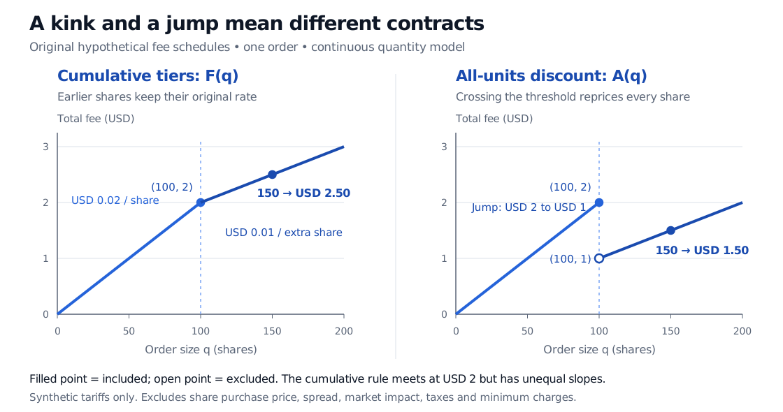
For the cumulative fee, both sides approach USD 2 at 100 shares. The total fee is continuous there. But its left slope is USD 0.02 per share and its right slope is USD 0.01 per share. Because these slopes disagree, the derivative at 100 does not exist: the graph has a kink.
That distinction matters when estimating marginal costs. For 0<h≤100, a centred difference gives
2hF(100+h)−F(100−h)=0.015.
The estimate is USD 0.015 per share even as the step shrinks. It averages the two slopes; it does not establish that a derivative exists. If orders must contain whole shares, use actual fee differences: moving from 100 to 101 shares adds USD 0.01. The calculus statement concerns the continuous extension specified above.
Now change the contract so that orders above 100 shares pay USD 0.01 on every share:
A(q)={0.02q,0.01q,0≤q≤100,q>100.
Then A(100)=2, while the right-hand limit at 100 is 1. These unequal one-sided limits create a jump, so A is discontinuous there. No choice of the single value A(100) can make those limits agree. This hypothetical all-units discount even makes a 101-share order cheaper in total than a 100-share order: USD 1.01 versus USD 2.00. Such a result must come from the stated tariff, not an accidental omission of the carried-forward charge.
Two hypothetical fee contracts plotted against order size in shares. Cumulative tiers meet at USD 2 for 100 shares and reach USD 2.50 at 150, with slopes 0.02 and 0.01 USD per share. An all-units discount has a filled point at 100 shares and USD 2, an excluded right-branch endpoint at USD 1, and a fee of USD 1.50 at 150.
Original synthetic tariffs for one order, in USD. The left contract has a continuous kink; the right contract has a jump. Filled and open markers distinguish included and excluded boundary points.
Piecewise definitions need not create either feature. For example, g(x)=x2 for x≤0 and g(x)=x3 for x>0 is continuous and differentiable at zero, with derivative zero. Different formulas can join without a corner. What matters is their values and limiting slopes at the join, rather than the fact that they occupy separate lines in a definition.
James Stewart, Single Variable Calculus: Early Transcendentals, 6th ed., Brooks/Cole, 2008: §1.1, piecewise-defined functions; §2.5, continuity; §2.8, differentiability and continuity.
Gilbert Strang and Edwin Herman, Calculus Volume 1, OpenStax: §1.1, Review of Functions, for functions, domains and piecewise notation.
OpenStax, §2.4, Continuity, for continuity conditions and jump discontinuities.