Multivariable calculus studies change and accumulation for functions with several inputs. In quantitative finance, it lets you combine individual price sensitivities into a joint scenario, integrate payoffs over several uncertain factors, and optimise portfolios subject to constraints. A multivariable function supplies the input–output relationship; calculus supplies the methods for analysing it. MIT's multivariable calculus course covers its differential, integral and vector branches.
The practical question is often: if several inputs move together, how much does the output change? A partial derivative answers only one part of that question by varying one input and holding the others fixed.
Two inputs move, and their effects oppose
Consider the present value of a certain payment of USD 100, with continuous discounting:
Here is the annual continuously compounded discount rate, entered as a decimal, and is remaining time to payment, in years. This is a synthetic two-input model with a single constant discount rate. The payment amount, currency, certainty and compounding convention remain fixed; there are no coupons, credit losses or transaction costs. At a fixed valuation date, varying compares payment horizons. Interpreting a reduction in as the passage of time instead changes the valuation date for the same payment.
At and , value is USD 88.692044. The first partial derivatives are
| Local sensitivity at the starting point | Value | What stays fixed |
|---|---|---|
| −266.076131 USD per unit of decimal annual rate | Remaining maturity years | |
| −3.547682 USD per year of remaining maturity | Rate |
A unit of decimal rate is much larger than a normal rate bump: one basis point is 0.0001, so a 10-basis-point rise is . It takes the quoted rate from 4% to 4.1%.
Now raise the rate by those 10 basis points and reduce remaining maturity by year. Because this function is differentiable, its gradient combines the two local effects:
The higher discount rate lowers value; the shorter wait increases it. Both derivatives are evaluated at the same starting point. This linear approximation is the finite-scenario use of the total derivative; it is not an exact finite repricing. MIT's tangent-approximation material develops the geometry behind this step.
Re-evaluating the model at both new coordinates gives
The new value is USD 88.789659. The first-order estimate misses USD 0.008923. That is small in dollars here, but noticeable relative to the net gain because two larger effects partly cancel.
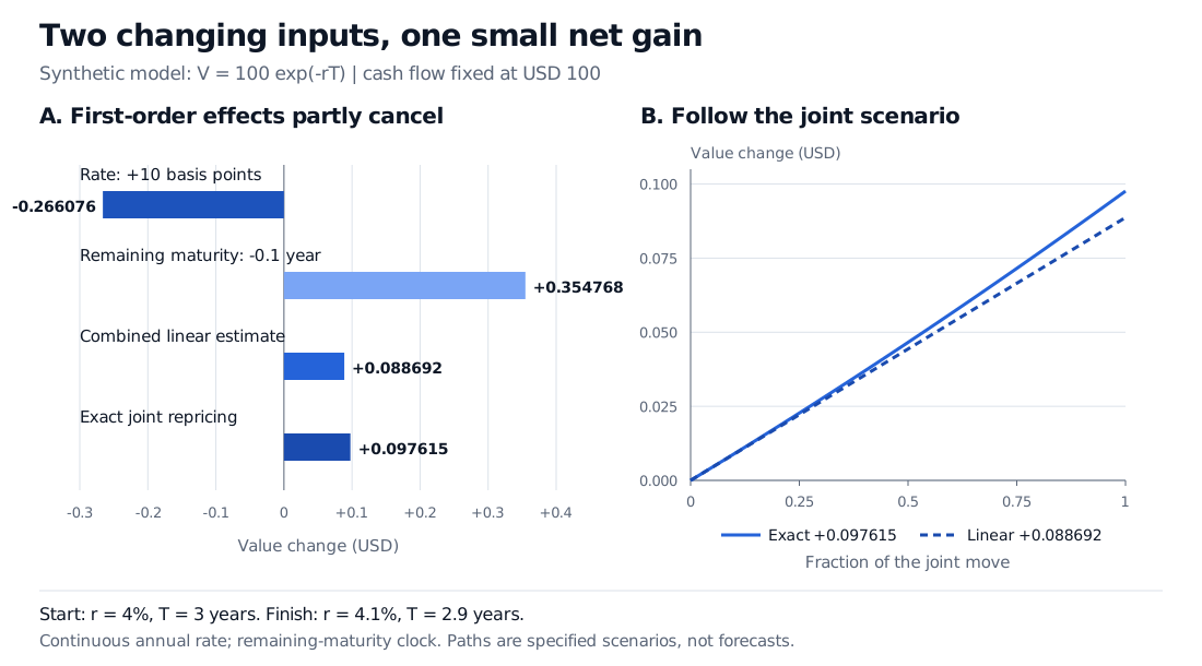
Original synthetic example with continuous annual discounting. The right panel follows the specified rate and remaining-maturity moves together; it is not a forecast or a market time series.
Interactions live beyond first order
The Hessian matrix collects second partial derivatives. For this model,
At the starting point, the mixed partial is −78.048998 USD per unit of decimal annual rate per year. It measures how the rate sensitivity changes when remaining maturity changes. Mixed partials agree in either order here because the function has continuous second derivatives.
The second-order approximation adds
For this scenario, that correction is USD 0.008914, bringing the estimated change to USD 0.097606. The mixed term is positive because while . The improved estimate still has a residual: a Taylor expansion truncated at second order does not capture every finite-change term.
Keep the clock explicit. measures increasing remaining maturity. For the same fixed payment as calendar time advances, when both clocks use years. At a fixed rate, the chain rule therefore gives , the opposite sign. If the rate also follows a differentiable path, the total rate of change is . A partial maturity sensitivity alone is not the realised change. At negative discount rates the maturity and calendar-time signs reverse; the calculus does not require a positive rate.
Sensitivities, integration and decisions
Differentiation is one branch. A double integral can aggregate a payoff against the joint density of two risk factors. Unlike the fixed scenario above, that calculation requires a probability model, including dependence, and suitable integrability. Two sensitivities alone do not supply those probabilities.
Optimisation uses derivatives to study how changing decision variables improves an objective. A zero gradient at an interior point is only a candidate condition; curvature, constraints and boundaries determine what can be concluded. A pricing input such as an interest rate is not automatically a variable the investor controls.
For a first guided treatment, the Partial Derivatives lesson develops fixed-input sensitivities, gradients and the distinction between a weight change and a fully invested reallocation. Its public preview is open; the full lesson requires membership.
Sources
-
Stanford University Mathematics Department, Linear Algebra, Multivariable Calculus, and Modern Applications, MATH 51 course text, version dated 10 March 2021: §9.2 for partial derivatives, §11.1 for local linear approximation, and §25.3 for quadratic approximation.
-
John C. Hull, Options, Futures, and Other Derivatives, 9th Global Edition, §4.2, continuous compounding and discounting. The payment example, calculations and figure here are original.
-
MIT OpenCourseWare, 18.02SC Multivariable Calculus, Fall 2010 — differential, integral and vector calculus.
-
MIT OpenCourseWare, tangent approximation and optimisation and chain rule, gradient and directional derivatives — the relationship between coordinate sensitivities and joint changes.
-
William L. Silber, NYU Stern: Continuous Compounding — continuous-rate discount factors and their distinction from annual compounding.