Double integral: Definition & Examples

A double integral adds the values of a function over a two-dimensional region, weighting each small piece by its area. It extends a definite integral from a line interval to a region in the plane:

\iint_D g(x,y)\,dA, \qquad dA=dx\,dy.

For a risk model driven by two uncertain quantities, that region can describe combinations of outcomes: both drivers below a threshold, a combined loss above a limit, or states in which a contract pays. Integrating a joint density over the region gives its probability; integrating payoff times density gives its expected payment. The region and the function being integrated answer different parts of the question.

From small cells to one number

Divide $D$ into small cells of area $\Delta A_{ij}$ . Evaluate $g$ at a point $(x_{ij}^*,y_{ij}^*)$ in each cell and add

\sum_{i,j}g(x_{ij}^*,y_{ij}^*)\Delta A_{ij}.

When these sums approach a common limit as the cells become finer, that limit is the double integral. For a continuous function on a closed rectangle this construction works. If

g\ge0

, its geometric interpretation is the volume under the surface

z=g(x,y)

and above

D

. A signed

g

instead gives a signed accumulation: negative contributions subtract. Taking

g=1

gives the area of

D

. OpenStax develops this construction.

The two integral signs do not mean “integrate the same expression twice in the same variable.” Each coordinate has its own range.

A quarter of the area, an eighth of the probability

Suppose a desk builds a synthetic model with two dimensionless risk-driver scores

X

and

Y

, each between zero and one. Higher scores represent larger adverse moves within this toy scenario. Assume the joint probability density

f_{X,Y}(x,y)= \begin{cases} x+y, & 0\le x\le1,\ 0\le y\le1,\\ 0, & \text{otherwise}. \end{cases}

This is an assumed teaching model, not an estimated market distribution. It is nonnegative and normalised:

\int_0^1\int_0^1(x+y)\,dy\,dx =\int_0^1\left(x+\frac12\right)dx =1.

The desk asks for the probability that both scores are at most 0.5. The event is the lower-left square

D=[0,0.5]\times[0,0.5]

. Read the innermost differential first: integrate in

y

, treating

x

as fixed, then integrate the resulting function in

x

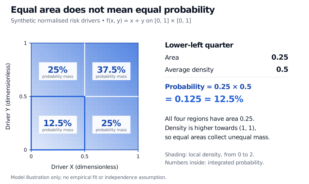
\begin{aligned} \mathbb{P}(X\le0.5,\ Y\le0.5) &=\int_0^{1/2}\int_0^{1/2}(x+y)\,dy\,dx\\ &=\int_0^{1/2}\left(\frac{x}{2}+\frac18\right)dx\\ &=\left[\frac{x^2}{4}+\frac{x}{8}\right]_0^{1/2}\\ &=\frac1{16}+\frac1{16}=\frac18=12.5\%. \end{aligned}

The region has area

0.25

, but its average density is

0.5

, giving probability

0.25\times0.5=0.125

. Assuming probability equals area would silently replace the stated density with a uniform one. The MIT joint-distribution notes distinguish density from probability and explain why probabilities require integration.

Synthetic joint density x plus y on the unit square. Four equal-area quadrants have masses 12.5%, 25%, 25% and 37.5%. The lower-left square has area 0.25 and average density 0.5, so its probability is 0.125.

Original synthetic model, with dimensionless coordinates. Shading represents local density; the percentages represent probability integrated over each quadrant. No empirical fit or independence assumption is used.

Density itself need not lie below one: here it reaches two. Probability is dimensionless and bounded by one; density has reciprocal coordinate-area units. If coordinates were measured in dollars and percentage points, the joint density would be per dollar per percentage point. A density value at one point is not the probability of that exact pair; under this joint density, any single point has probability zero.

Two integrations do not assume independence

Integrating out

Y

gives the marginal distribution of

X

, with density

f_X(x)=\int_0^1(x+y)\,dy=x+\frac12, \qquad 0\le x\le1.

It is not uniform. By symmetry,

f_Y(y)=y+1/2

on the same interval. Their product is generally different from

x+y

, so

X

and

Y

are not independent.

Indeed, each individual probability below 0.5 is $3/8$ . Multiplying them gives $9/64$ , whereas the correct joint probability is $1/8=8/64$ . Computing two successive integrals is a method for adding the joint density; multiplying marginal probabilities requires a separate independence justification.

Reversing the order means preserving the region

For a continuous $g$ on a rectangle $[a,b]\times[c,d]$ , Fubini's theorem permits either order:

\int_a^b\int_c^d g(x,y)\,dy\,dx =\int_c^d\int_a^b g(x,y)\,dx\,dy.

The same principle works beyond continuous rectangle examples with suitable conditions. For a nonnegative measurable integrand, Tonelli's theorem permits either order, possibly with an infinite result. For a signed integrand, absolute integrability is a sufficient condition:

\iint_D\lvert g(x,y)\rvert\,dA<\infty.

These are conditions on the integral, not assumptions about independence. Warnick's Cambridge notes state both results, Appendix B.3.2. Our density is bounded on a finite square, so no convergence issue arises.

For a nonrectangular event, changing order also changes the limits. For example, the triangle $D=\{x\ge0,y\ge0,x+y\le1\}$ can be written either way:

\iint_D g(x,y)\,dA =\int_0^1\int_0^{1-x}g(x,y)\,dy\,dx =\int_0^1\int_0^{1-y}g(x,y)\,dx\,dy.

Replacing those inner limits by one would integrate over the entire square and include outcomes outside the event. Sketching the region before evaluating is often more useful than immediately finding an antiderivative.

Change the integrand to change the question

Under the same joint density, the expected value of a function

h(X,Y)

\mathbb{E}[h(X,Y)] =\int_0^1\int_0^1h(x,y)(x+y)\,dy\,dx,

provided its absolute expectation is finite. A probability uses the density over an event; an expectation additionally weights each state by its outcome. The University of Texas notes show this distinction and the marginalisation formulas.

For example, imagine a hypothetical payment of USD $12{,}000XY$ at the scenario horizon. Its expected payment is

\begin{aligned} \mathbb{E}[12{,}000XY] &=12{,}000\int_0^1\int_0^1xy(x+y)\,dy\,dx\\ &=12{,}000\left(\frac16+\frac16\right) =\text{USD }4{,}000. \end{aligned}

The currency units come from the payment function; density times coordinate area supplies a probability weight. This is an expected payment under the assumed scenario distribution. Turning it into a traded contract's price would additionally require appropriate valuation probabilities and discounting. Integrating the payment alone would omit the model's probability weights.

For a fuller treatment of probabilities, marginals and conditional densities, see Joint Densities, Marginals, and Conditioning. The link opens a public preview; the complete lesson requires membership.

Sources

Steven G. Krantz and Harold Parks, Vector Calculus, first edition, CRC Press, 2024, §4.1, especially Theorem 4.1.6: double Riemann sums and iterated integration for continuous functions on rectangles.
Dimitri P. Bertsekas and John N. Tsitsiklis, Introduction to Probability, second edition, Athena Scientific, 2008, §3.4: joint densities, probabilities and marginal densities.
OpenStax, Calculus Volume 3, §5.1: rectangular double integrals and geometric interpretation.
Jeremy Orloff and Jonathan Bloom, MIT 18.05, Reading 7a: Joint Distributions, Independence, §§3.2 and 5: joint density and independence.
Claude Warnick, Analysis of Functions, Cambridge, 2021, Appendix B.3.2, Theorems B.29–B.30: Tonelli and Fubini.
University of Texas at Austin, Double Integrals in Probability: moments and marginal distributions.

The risk-driver model, payment example and figure are original synthetic illustrations.

From small cells to one number

A quarter of the area, an eighth of the probability

Two integrations do not assume independence

Reversing the order means preserving the region

Change the integrand to change the question

Sources

Related terms

Definite integral

Expected value

Independence

Marginal distribution

Probability density function