Distinguish the most frequent sample value, a discrete probability mode and a continuous density peak, with tied counts and a binning counterexample.
Mode
The mode is a value with the greatest observed frequency in a sample, or the greatest probability mass in a discrete population model. For a continuous model, a mode maximises a specified probability density. A mode need not be unique, and its location is different from the frequency, probability or density height used to identify it.
For a desk monitoring rejected orders, the mode answers “Which count occurred most often?” It does not answer “What was the average count?” or “How large could the next count be?”
The most common outcome can differ from the average
Suppose a synthetic credit model assigns the following probabilities to the number N of defaults in a two-loan pool over one year:
Defaults n
Probability P(N=n)
0
0.50
1
0.30
2
0.20
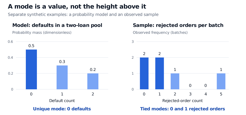
The unique mode is 0 defaults, because 0.50 is the largest probability mass. The mode is not 0.50: that is its probability. Meanwhile, the expected value is
E[N]=0(0.50)+1(0.30)+2(0.20)=0.70.
An expected count can be fractional even though an actual default count cannot. “No defaults” is the single most probable outcome here, but some defaults occur with total probability 0.50. Using the mode alone to budget credit losses would discard that part of the model.
Now consider a separate synthetic operational sample: rejected-order counts across six batches are 0,0,1,1,2,5. Both 0 and 1 occur twice, so both are sample modes. Each has relative frequency 2/6=1/3. The sample mean is 9/6=1.5 rejected orders per batch; it is neither a mode nor an observed count.
Separate synthetic examples: default-count probabilities are 0.50, 0.30 and 0.20 at counts 0, 1 and 2, giving mode 0. Rejected-order sample frequencies at counts 0 through 5 are 2, 2, 1, 0, 0 and 1, giving tied modes 0 and 1.
The horizontal position identifies a mode; the bar height explains why it is modal. These are separate examples, not a model and a sample drawn from it.
For observed values x1,…,xn, define the frequency of value v by
c(v)=i=1∑n1{xi=v}.
Every observed value attaining the largest c(v) belongs to the sample's set of modes. If all observations are distinct, every value ties under this maximiser definition. Many elementary conventions instead report “no mode.” Either way, there is no informative single most frequent value. State the convention when software returns a result for such a sample.
For the standard normal distribution, the unique mode is zero: its density is greatest there. Yet P(X=0)=0, just as at every other exact value. Probability comes from area over an interval. Calling zero the “most likely exact observation” hides this distinction.
Density modes refer to the variable's scale and the chosen density representation. Ordinary linear unit conversion rescales their locations and density heights consistently. A nonlinear transformation can move the peak because the transformed density includes a Jacobian factor; transforming a mode is not generally enough to find the new mode. A flat density can have an entire interval of maximisers. Several equally high peaks give several global modes; analysts also use “multimodal” for densities with several local peaks, even if their heights differ.
Bins can move the apparent peak
A histogram groups observations rather than counting exact repeated values. For the rejected-order sample, equal-width bins [−0.5,1.5), [1.5,3.5) and [3.5,5.5) contain 4, 1 and 1 observations. Shift the same width-two bins to start at −1.5: the four counts become 2, 3, 0 and 1. The tallest bin changes, while the raw-data modes remain 0 and 1.
A modal bin is therefore a feature of a particular grouping, not an exact population mode. With unequal bin widths, compare density heights when interpreting peaks, rather than treating the largest count as the tallest density. Smoothing choices likewise affect estimated peaks. These distinctions matter for execution latencies and returns, where rounding, tick sizes or binning can create an apparently precise “typical” value.
For a worked continuous example, Normal Distribution explains density height versus interval probability and why the mean, median and mode coincide in that particular family. The full lesson is free with a signed-in account; the public page provides a preview.
Sources
Blitzstein, J. K., and Hwang, J. Introduction to Probability, second edition, §6.1, Definition 6.1.2: discrete and continuous distribution modes.