A martingale difference has zero conditional mean given the past. An exact two-step model shows how predictable risk and dependence can survive zero serial covariance.
Martingale difference sequence
A martingale difference sequence is a sequence of integrable random variables whose next value has conditional expectation zero given the information available before it arrives. It describes successive surprises, such as errors from a correctly specified conditional-mean forecast. The surprises can have predictable risk even when their mean is unpredictable.
The information is part of the claim
Fix a probability measure P and a filtration(Ft)t≥0, where Ft represents information available after step t. A sequence (Dt)t≥1 is a martingale difference sequence relative to that filtration if, for each t:
Dt is Ft-measurable: it is an adapted process, observable by time t.
EP[∣Dt∣]<∞: the required means exist.
Almost surely,
EP[Dt∣Ft−1]=0.
The condition concerns the whole specified past, rather than only the immediately preceding value. Changing the information set or probability measure can change whether it holds. Bartlett gives this definition in Lecture 5, slide 17.
Why “difference”? If (Mt) is a martingale, then Dt=Mt−Mt−1 satisfies the condition. Conversely, starting from M0=0, the partial sums
Mt=j=1∑tDj
form a martingale, because E[Mt∣Ft−1]=Mt−1+0. The sequence of changes is the martingale difference sequence; the sequence of accumulated changes is the martingale. The changes themselves need not form a martingale.
Zero mean, changing risk
Consider a synthetic two-step model. Let ξ1,ξ2 be independent signs, each equally likely to be +1 or −1. Define two changes, measured in USD:
D1=ξ1USD,D2=(2+ξ1)ξ2USD.
Use the trivial initial information F0={∅,Ω}, then F1=σ(ξ1) and F2=σ(ξ1,ξ2). Each change is observable at its own time and bounded, so adaptedness and integrability hold. The first change has mean zero. For the second,
E[D2∣F1]=(2+ξ1)E[ξ2∣F1]USD=0.
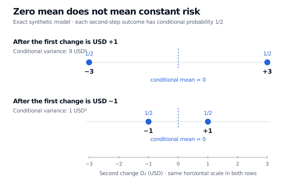
After an up first step, the next change is USD +3 or USD −3, each with probability 1/2. After a down first step, it is USD +1 or USD −1, again equally likely. Both conditional means are zero, while the conditional variance is
The conditional second change is USD minus 3 or plus 3 after a USD plus 1 first change, with variance 9 USD squared. After a USD minus 1 first change, it is USD minus 1 or plus 1, with variance 1 USD squared. Both conditional means are zero.
Original exact synthetic model. Each displayed pair has conditional probability one half per outcome. The shared horizontal scale shows changing risk around the same zero conditional mean.
The unconditional variance of D2 is the average (9+1)/2=5USD2. Its distribution is plainly different from that of D1, whose variance is 1USD2. Neither identical distributions nor constant conditional variance is required. Normality is not required either: this example has only four equally likely paths.
The accumulated process M0=0, M1=D1, M2=D1+D2 is a martingale. Its possible terminal values are USD 4,−2,0,−2, indexed by sign paths ++,+−,−+,−−. After the first up step, the two terminal values average to USD 1; after the first down step, they average to USD −1.
Uncorrelated can still mean dependent
With finite second moments, martingale differences at distinct times have zero covariance. For s<t, the earlier Ds is already known at time t−1, so
E[DsDt]=E[DsE[Dt∣Ft−1]]=0.
The unconditional means also vanish by total expectation. Hence Cov(Ds,Dt)=0. Finite second moments ensure the products are integrable; the definition alone only requires first absolute moments. These orthogonality and sum-of-variances results are developed in Lalley, §1.2.
In our example, Cov(D1,D2)=0, yet the changes are dependent. Seeing ∣D2∣=USD 3 reveals that D1=USD 1. Before seeing it, that first up step had probability 1/2; afterwards its conditional probability is 1. Zero covariance misses this dependence in magnitude.
Independent, mean-zero, integrable variables are a sufficient construction relative to their natural filtration. Independence is a stronger assumption than the martingale-difference condition. Merely observing zero serial covariance is weaker and cannot establish the condition.
Forecasting the mean and forecasting the risk
For any integrable adapted outcome Yt, subtracting its true conditional mean gives
Dt=Yt−E[Yt∣Ft−1],
a martingale difference sequence. An estimated model's residuals need not have this property: its forecast may omit relevant past information or estimate the conditional mean poorly.
This distinction matters for financial returns. A conditional-mean model can leave no forecastable mean in its errors while a volatility model still predicts their scale. The martingale-difference assumption therefore leaves room for time-varying conditional risk; it does not establish that raw returns have zero conditional mean, nor does it specify a complete trading-profit model.
For worked conditional averages, the tower property and the forecast-error identity, use SelfMadeQuant's Conditional Expectation lesson (public preview; full lesson requires membership).
Practice: is zero covariance enough?
Let Z take values −1,0,1 with equal probability. Set A=2ZUSD and B=(3Z2−2)USD. First reveal A, then B, using the trivial initial information and the natural filtration of these two changes. Both changes have mean zero and Cov(A,B)=0. Do they form a martingale difference sequence?
Answer. No. Observing A reveals Z, so B is already determined. If A=0, then E[B∣A]=USD (−2); if A=USD (±2), that conditional mean is USD 1. Neither is zero. The unconditional mean of B is (1−2+1)/3=0, and the product mean is (−2+0+2)/3=0USD2, but averaging across histories hides the predictable second change.
Alexander J. McNeil, Rüdiger Frey and Paul Embrechts, Quantitative Risk Management: Concepts, Techniques and Tools, revised edition, Princeton University Press, 2015, §4.1.1, Definition 4.6: information-relative martingale differences, zero autocovariance and the additional constant-variance requirement for weak white noise.