The half-width of a symmetric confidence interval: calculate a slippage margin, separate it from standard error, and see why more data cannot remove every error.
Margin of error
A margin of error is the distance from a point estimate to either endpoint of a symmetric confidence interval. If the interval is reported as “estimate plus or minus m,” then m is its margin of error and 2m is its full width. It expresses sampling uncertainty at a specified confidence level, under a specified method and model.
For an execution researcher, “average slippage 5.2 basis points” is incomplete without a precision statement. A margin of 0.49 bp says something useful about uncertainty in average slippage. It does not say that each order's slippage stays within 0.49 bp of that average, or that the estimated average can never be wrong by more than 0.49 bp.
From an error scale to an interval
For many familiar symmetric intervals,
m=c×SE(θ^),[θ^−m,θ^+m].
The standard error is the sampling standard deviation of the estimator. The critical multiplier c supplies the interval's confidence level and depends on the reference distribution. The margin and the standard error share the parameter's units; the critical multiplier is dimensionless.
Consider synthetic summary statistics, with slippage measured relative to a fixed arrival-price benchmark and positive values meaning worse execution. Stipulate that the observations are independent normal draws with a constant unknown mean μ and a known population standard deviationσ=1.5 bp. The sample size and analysis are fixed in advance. These assumptions make this a transparent exact calculation; they are not automatic properties of transaction data.
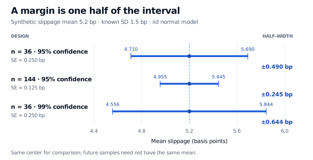
The 95% interval is approximately 4.710 to 5.690 bp. Its full width is about 0.980 bp; the margin is 0.490 bp. The population SD of 1.5 bp describes individual-order dispersion, the SE of 0.25 bp describes mean-estimation variability, and the margin attaches the chosen confidence level to that variability.
If σ were estimated by the sample SD s, the exact iid normal-mean construction would instead use a Student t distribution: m=tn−1,1−α/2s/n. A historical volatility estimate does not become a known population SD simply because it is entered into a formula.
More observations or more confidence?
Hold the model and population SD fixed. Two changes pull precision in opposite directions:
Design
SE (bp)
Margin (bp)
Interval if the mean remains 5.2 bp
36 observations, 95% confidence
0.250
0.490
4.710 to 5.690 bp
144 observations, 95% confidence
0.125
0.245
4.955 to 5.445 bp
36 observations, 99% confidence
0.250
0.644
4.556 to 5.844 bp
Three symmetric intervals centered at synthetic mean slippage 5.2 bp: 36 observations at 95% gives margin 0.490 bp; 144 at 95% gives 0.245 bp; 36 at 99% gives 0.644 bp.
Original hypothetical comparison under an iid normal model with known SD 1.5 bp. The center is held fixed to isolate width changes; an actual new sample would generally change the mean.
Quadrupling the sample size halves this margin because it scales as 1/n. Raising confidence from 95% to 99% uses z0.995≈2.575829 and widens the interval without changing the SE. A narrower margin bought by lowering confidence is a weaker coverage claim, not improved data.
Under this exact model, the probability before sampling that the absolute mean-estimation error is at most m equals the chosen confidence level. Across repeated 36-observation samples, the 95% interval procedure covers the fixed mean 95% of the time. A particular observed interval either covers it or does not. The margin is therefore not a guaranteed maximum error; normal sampling error has unbounded tails.
Nor is it a budget for every source of uncertainty. If the data omit difficult-to-fill orders, the sample can target the wrong execution population. A misrecorded arrival benchmark can shift the estimate. Choosing only a favorable venue or period after inspection changes the analysis. More observations may shrink the printed margin while leaving sampling bias, measurement error or selection effects intact. Dependence across orders and a changing execution regime also undermine the stated iid constant-mean model.
Finally, not every interval has one common margin around the point estimate. For an asymmetric interval [L,U], report the endpoints or separate distances θ^−L and U−θ^ when the estimate lies inside it. Reporting (U−L)/2 alone conceals the asymmetry: that is a half-width around the interval's midpoint, which need not be the estimate. Variance intervals and intervals transformed onto a nonlinear scale provide familiar examples. Always state the parameter, confidence level and construction alongside a margin.
Sources
John A. Rice, Mathematical Statistics and Data Analysis, 3rd ed. (2007), §8.5.3, pp. 279–280: coverage, the exact normal-mean t interval, and the asymmetric variance interval; §9.2, p. 333: known-variance normal sampling law. The slippage example and figure are original.