An interarrival time is the elapsed time between two consecutive events. If is the time of event , its interarrival time is . Arrival times are clock readings; interarrival times are durations.
For a quant studying order messages, trades or credit events, this distinction turns timestamps into a sequence of waits. The sequence can reveal changing activity or clustering that a single daily count conceals. An event must first be defined consistently: a quote update and a completed trade are different things to count.
Read the gaps, then read the stopping rule
Consider a synthetic record of qualifying events. Start the clock at an observed event, , and record subsequent events at 0.4, 1.1 and 1.6 hours. Observation ends at the predeclared time 2 hours. The origin event anchors the clock; it is not counted as a new event in .
| Consecutive events | Completed interarrival time |
|---|---|
| 0 to 0.4 hours | 0.4 hours = 24 minutes |
| 0.4 to 1.1 hours | 0.7 hours = 42 minutes |
| 1.1 to 1.6 hours | 0.5 hours = 30 minutes |
The sample mean of the three completed gaps is
From the last event to the end of observation, another 0.4 hours pass without an event. This is a right-censored wait: we know hours, but do not know its eventual length. Calling it a fourth completed gap would replace an unknown duration with its observed lower bound. Omitting it from a rate calculation would discard exposure during which no event occurred.
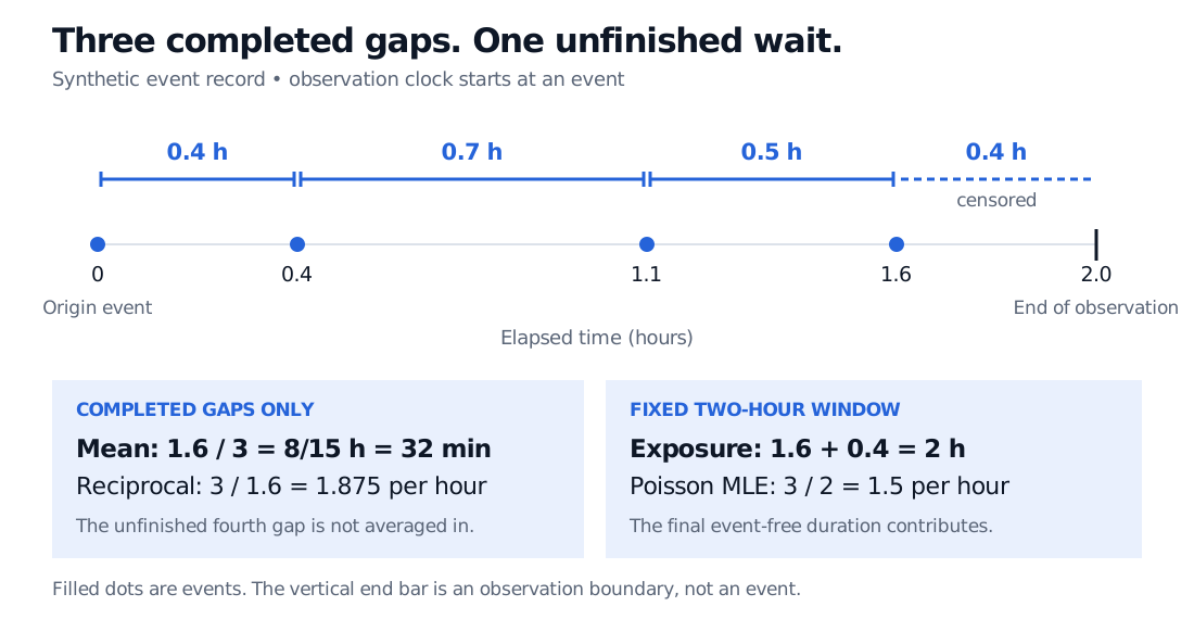
Original synthetic timeline. Filled dots are events; the end bar marks the observation boundary. The final 24 minutes contribute exposure, although they do not complete another gap.
A probability law needs an assumption
The definition of an interarrival time does not imply a particular distribution or independence. Under a homogeneous Poisson process with constant rate , the successive gaps are independent and identically distributed with an exponential distribution:
As a separate stipulated model, take events per hour. The theoretical mean gap is 0.5 hours, or 30 minutes, and the probability that a gap exceeds half an hour is , about 36.79%. These are model quantities, not estimates obtained from the three synthetic gaps. Rates have inverse-time units; the product is dimensionless.
For the construction linking independent exponential gaps to event counts, Defining the Poisson Process: Three Equivalent Constructions has a public preview; the full lesson requires membership.
Why the two rate calculations differ
The reciprocal of the completed-gap average is
That is the exponential rate maximum likelihood estimate for a design that records three complete waits and stops at the third arrival. Our stated design instead continues to a fixed two-hour endpoint.
Under the homogeneous Poisson model, each completed wait contributes a density factor . The unfinished wait contributes a survival factor . Multiplying gives the likelihood, conditional on the origin event,
All durations here are expressed in hours. The log-likelihood, up to a parameter-independent constant, is . Its derivative vanishes at
The same maximiser follows from the Poisson distribution for the three events counted in the full window. The lower rate reflects the additional event-free exposure. It does not contradict the 32-minute completed-gap average: the two calculations use different observation endpoints. The survival contribution follows the usual likelihood treatment of censored observations.
In real records, also check the beginning of the window. If observation starts between events and the preceding event time is unknown, the first observed delay is a forward waiting time, not a measured full interarrival gap. These have the same exponential law in the homogeneous Poisson case, but need not have the same law more generally. Time-of-day effects, dependence between arrivals and timestamp resolution all matter before treating observed gaps as independent exponential data.
Sources
- Richard Durrett, Essentials of Stochastic Processes, third edition (2016), §§2.1–2.2, especially the exponential moments and construction from independent exponential gaps.
- Robert G. Gallager, Poisson Processes, Chapter 2 of MIT stochastic-process notes, §§2.1–2.2 — arrival epochs, interarrival intervals, counting processes and waiting from a fixed observation time.
- NIST/SEMATECH e-Handbook of Statistical Methods, §8.4.1.2: Maximum likelihood estimation — density and survival contributions and exponential-rate estimation from total exposure.