Higher-order derivative: Definition & Examples

A higher-order derivative is a derivative taken repeatedly: the second derivative measures how the first derivative changes, the third measures how the second changes, and so on. In pricing, these orders distinguish a position's immediate sensitivity from the way that sensitivity changes as a market input moves.

An order is a new rate of change

Starting with a derivative

f'

, define

f''(x)=\frac{d}{dx}f'(x),\qquad f'''(x)=\frac{d}{dx}f''(x),\qquad f^{(n)}(x)=\frac{d}{dx}f^{(n-1)}(x).

The notation

f^{(n)}

means differentiate

n

times. It does not mean raise

f'

to the power

n

: if

f(x)=x^2

, then

f''(x)=2

, whereas

[f'(x)]^2=4x^2

. Likewise,

d^2f/dx^2

denotes repeated differentiation, not a squared fraction.

Each order needs its own existence condition. A function having a first derivative does not guarantee that it has a second. Where $f''$ is positive throughout an interval, $f'$ is increasing there; that says nothing by itself about whether $f'$ is positive. A price can fall while its slope becomes less negative.

Units also change with order. If $f$ is measured in USD and $x$ in a chosen input unit, then $f^{(n)}$ has units USD per input-unit to the power $n$ . Comparing raw first- and second-derivative magnitudes without their units is misleading.

Three corrections to the same bond move

Consider a hypothetical fixed payment of USD 100 in two years, discounted at a continuously compounded annual yield

y

expressed as a decimal. Holding the payment and maturity fixed, its present value is

P(y)=100e^{-2y}.

Repeated use of the chain rule gives

P'(y)=-2P(y),\qquad P''(y)=4P(y),\qquad P'''(y)=-8P(y),\qquad P^{(n)}(y)=(-2)^nP(y).

y_0=0.05

, the price is USD

90.483742

. The first three derivatives are approximately

-180.967484

361.934967

, and

-723.869934

, with units USD per annual decimal-yield unit, per squared unit, and per cubed unit respectively. The negative first derivative means a higher yield lowers price; the positive second derivative means the price–yield curve has positive convexity. These signs are entirely compatible. The negative third derivative means that this dollar curvature decreases as yield rises.

Now raise yield from 5% to 6%:

h=0.01

, or 100 basis points. A Taylor expansion adds successive corrections to the predicted price change:

\Delta P\approx P'(y_0)h+ \frac{P''(y_0)}{2!}h^2+ \frac{P'''(y_0)}{3!}h^3.

The linear term is USD $-1.809674836$ . The second-order correction adds USD $0.018096748$ ; the third-order correction subtracts USD $0.000120645$ . The factorials matter: a second derivative is not itself the quadratic coefficient.

Terms retained	Estimated change (USD)	Absolute error against repricing (USD)
First order	−1.809674836	0.017976704
First + second	−1.791578088	0.000120044
First + second + third	−1.791698733	0.000000601
Exact repricing	−1.791698132	0

Exact repricing means evaluating $100e^{-0.12}-100e^{-0.10}$ directly. The second-order estimate slightly understates the loss; the third-order estimate slightly overstates it. All values concern this synthetic payment, before transaction costs or other risks.

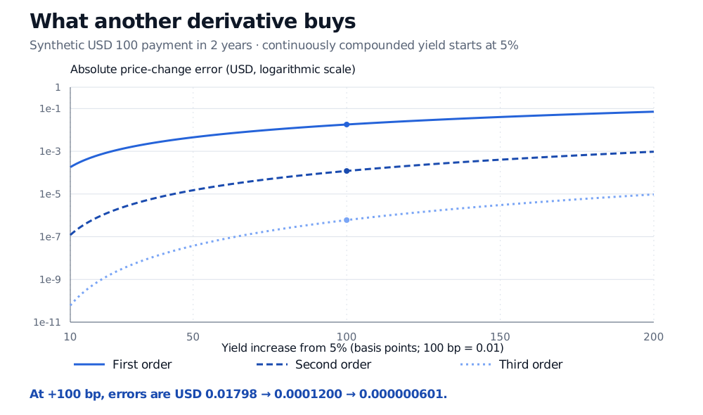
Absolute price-change errors for a synthetic USD 100 two-year payment when yield rises from 5% by 10 to 200 basis points. At 100 basis points, first-, second- and third-order errors are USD 0.017976704, USD 0.000120044 and USD 0.000000601. Higher orders reduce error throughout the plotted range; the vertical axis is logarithmic.

Original synthetic example. Each curve retains all terms through the stated order, using derivatives at 5%. The vertical axis shows absolute error in USD on a logarithmic scale.

Entering $h=1$ for a one-percentage-point move would instead mean a 100-percentage-point move under this decimal-yield convention. If the input is changed to percentage-number units $z=100y$ , the $n$ th derivative becomes $100^{-n}P^{(n)}(y)$ ; its product with the corresponding $n$ th-power input change remains the same monetary correction.

Higher order still needs an error argument

For a function with continuous derivatives through order $n+1$ on the interval between $a$ and $a+h$ , Taylor's theorem gives

f(a+h)=\sum_{k=0}^{n}\frac{f^{(k)}(a)}{k!}h^k+R_n, \qquad |R_n|\leq\frac{M|h|^{n+1}}{(n+1)!},

where $f^{(0)}=f$ and $M$ bounds $|f^{(n+1)}|$ across that interval. The next derivative evaluated only at the starting point is not generally such a bound.

For this bond's upward move, $|P^{(4)}(y)|=16P(y)$ decreases with yield. Hence $M=16P(y_0)$ bounds the fourth derivative from 5% to 6%, and the third-order price error is at most USD $0.000000603225$ . The observed error, about USD $0.000000600820$ , satisfies that bound.

This unusually smooth example supports very accurate local corrections. A finite Taylor polynomial is not an exact revaluation in general; adding one more term does not guarantee improvement for every function and every finite move. Near a kink, a required higher derivative may not exist. For a pricing model with several changing inputs, separate single-variable orders also omit mixed effects: partial derivatives are needed to track those interactions.

To practise repeated differentiation, the polynomial and exponential derivatives lesson develops the rules and includes a section on higher derivatives of polynomials. Its public page is a preview; the full lesson requires membership.

Sources

James Stewart, Single Variable Calculus: Early Transcendentals, sixth edition, §2.8 “The Derivative as a Function,” higher derivatives; §§11.10–11.11, Taylor polynomials and error estimates.
NIST Digital Library of Mathematical Functions, §1.4(iii), Higher Derivatives: recursive definition and notation.
MIT OpenCourseWare, 18.100A, Lecture 20: Taylor's Theorem: finite Taylor polynomials and the remainder theorem.

An order is a new rate of change

Three corrections to the same bond move

Higher order still needs an error argument

Sources

Related terms

Basis point

Chain rule

Convexity

Derivative (calculus)

Partial derivative

Present value