An empirical distribution is the probability distribution that assigns equal weight to each observation in a sample. If a return occurs twice, it receives twice the mass of a return that occurs once. It turns a historical return series into a distribution from which you can calculate event frequencies, averages and resampled scenarios, without first choosing a normal or other parametric model.
The word empirical matters: these probabilities describe the sample. Treating them as estimates of future probabilities requires a defensible connection between the sampled data and the future market.
Five days, four distinct returns
Consider five illustrative daily returns, recorded in percent:
Each row gets probability . Combining equal values gives this probability mass function:
| Daily return | Number of rows | Empirical probability |
|---|---|---|
| −2% | 1 | 0.2 |
| −1% | 1 | 0.2 |
| 0% | 2 | 0.4 |
| +3% | 1 | 0.2 |
The empirical probability of a negative day is . The probability of a return strictly above 1% is . The expected value under this distribution equals the sample arithmetic mean:
This is a mean daily return, not a compounded return over the five days. Nor does a zero mean imply that there were no losses.
Giving each of the four distinct values probability would build a different distribution. It would underweight the repeated zero and overweight every other value. In this particular example even that incorrect distribution has mean zero, so checking only the mean would miss the mistake.
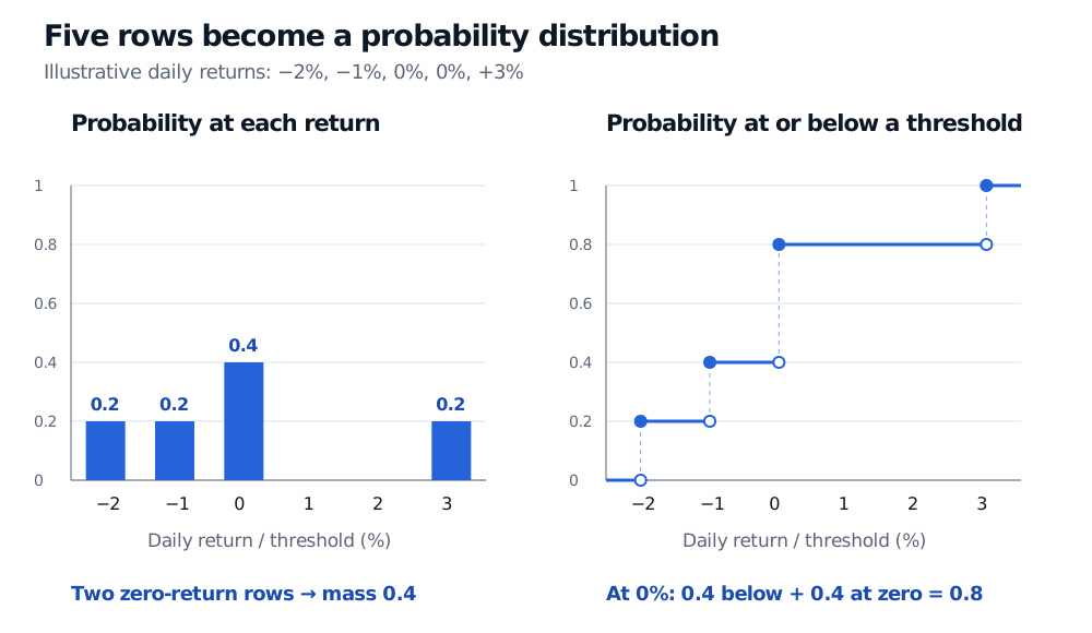
The left panel shows mass at each distinct value; the right panel accumulates it. Filled points include the endpoint, while hollow points exclude it. Original illustrative data, not observed market returns.
The distribution and its cumulative view
For observations with , the empirical probability of an event is
The indicator function counts the rows satisfying the event. This definition works for repeated values and does not require the underlying population to be discrete.
Its cumulative distribution function, often called the empirical CDF, is
For our returns, : both losing days and both zero-return days count. This differs from the 0.4 probability of a strictly negative return. At a value appearing times, the cumulative curve jumps by . It includes that jump at the value itself and stays constant until the next observed value. See Yen-Chi Chen's lecture on empirical distributions and statistical functionals.
A finite empirical distribution is always discrete, even when the data came from a continuous population. A histogram groups observations into bins; a fitted density smooths or models them. Neither is the same object as the raw empirical distribution. Cosma Shalizi's density-estimation lecture illustrates these distinctions.
Resampling the rows
An ordinary nonparametric bootstrap draws observations independently with replacement from the empirical distribution, conditional on the recorded sample. Choosing a row uniformly is equivalent to drawing a value using the table's masses. Thus a bootstrap draw has a 0.4 probability of zero; two independent draws are both zero with probability .
A bootstrap sample of five rows can repeat a losing day and omit the winning day. Its mean can differ from zero, although every individual resampled return must be one of the recorded values. The distribution of those repeated sample means is a bootstrap distribution of a statistic; it is different from the empirical distribution of individual returns. Larry Wasserman's bootstrap chapter explains the resampling construction.
For a worked implementation and the distinction between Monte Carlo error and sampling uncertainty, read Simulation and Resampling (public preview; full lesson requires membership).
What the sample cannot establish
The empirical distribution puts zero mass below −2% in this example. That is a fact about these five recorded days, not evidence that larger future losses are impossible. Ordinary resampling cannot generate an individual return outside the observed range; drawing more bootstrap samples does not supply unseen crash observations.
For independent observations from a common distribution, the empirical CDF consistently estimates that distribution's CDF as sample size grows. A historical trading series can violate this sampling setup through changing regimes, serial dependence or sampling bias. The empirical distribution also discards time order: shuffling the five rows leaves it unchanged, despite order being relevant to path-dependent risk.
If recent observations receive larger weights, the result is a weighted empirical distribution. State those weights explicitly: equal row weights are no longer the rule, and ordinary uniform-row bootstrap sampling no longer reproduces that weighted law.
Sources
- Larry Wasserman, All of Statistics: A Concise Course in Statistical Inference (Springer, 2004), §§7.1–7.2 and Chapter 8: empirical CDF, plug-in estimation and bootstrap.
- Yen-Chi Chen, University of Washington: Statistical functionals and the bootstrap.
- Cosma Shalizi, Carnegie Mellon University: Density estimation, 21 March 2019.
- Larry Wasserman, Carnegie Mellon University: The Bootstrap, Chapter 11.