Empirical cumulative distribution function: Definition & Examples

The empirical cumulative distribution function (ECDF) gives the fraction of observed values at or below a threshold. It is the data-based counterpart of a cumulative distribution function: a desk can use it to count how often a strategy's recorded P&L was nonpositive, without fitting a normal distribution or choosing histogram bins.

For observations $x_1,\ldots,x_n$ , with $n\ge1$ , define

F_n(x)=\frac{\#\{i:x_i\le x\}}{n} =\frac1n\sum_{i=1}^n\mathbf{1}_{\{x_i\le x\}}.

Each indicator contributes one if its observation qualifies and zero otherwise. The threshold has the observations' units; the output is a unitless proportion between zero and one. Constructing this descriptive curve requires no independence assumption. Interpreting it as an estimate of a population distribution does require a sampling model.

Three observations qualify; only one is negative

Consider five synthetic one-period P&L observations, in USD:

-2,\quad 0,\quad 0,\quad 3,\quad 5.

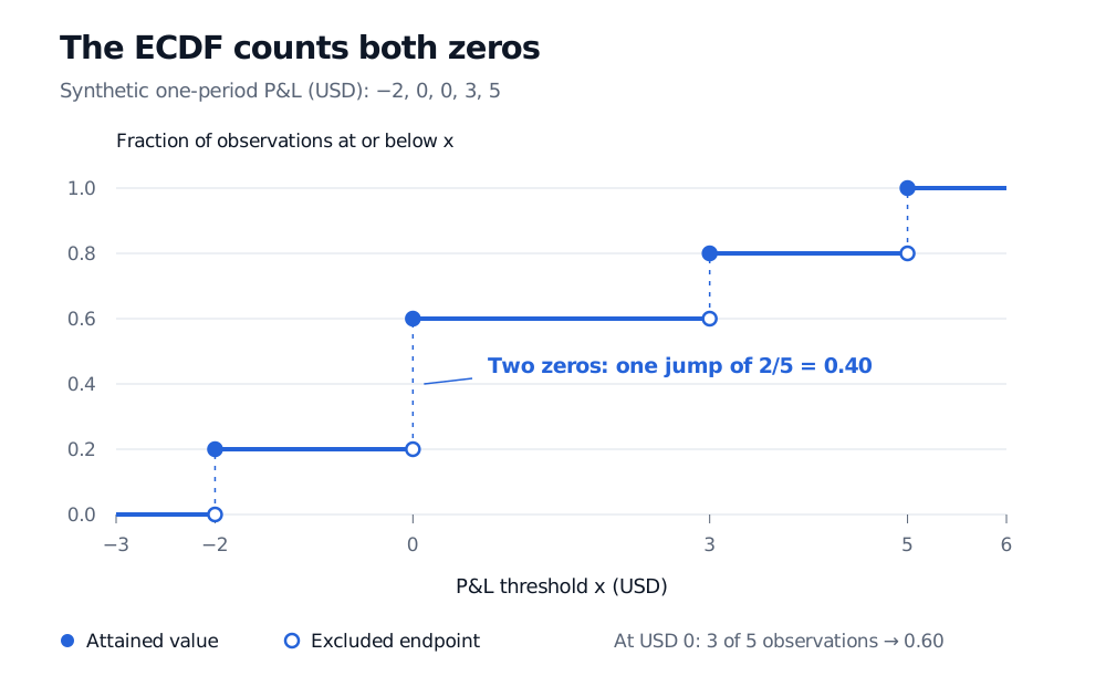
At a threshold of USD 0, the negative observation and both zeros qualify, so $F_5(0)=3/5=0.60$ . Immediately below zero, only USD −2 qualifies: $F_5(0-)=1/5=0.20$ . The two tied observations create a single jump of $2/5=0.40$ .

The entire curve is

F_5(x)=\begin{cases} 0,&x<-2,\\ 0.20,&-2\le x<0,\\ 0.60,&0\le x<3,\\ 0.80,&3\le x<5,\\ 1,&x\ge5, \end{cases}

where

x

is measured in USD. Every distinct observed value starts a step that includes its left endpoint. This is right continuity: the function's value at a jump is its value just to the right. A value occurring

r

times produces a jump of

r/n

, rather than

1/n

Five synthetic one-period P&L observations in USD are minus 2, 0, 0, 3 and 5. The ECDF is zero below minus 2, 0.2 from minus 2 to below zero, 0.6 from zero to below 3, 0.8 from 3 to below 5, and one at 5 and above. At zero, a filled point at 0.6 includes both zeros; a hollow point at 0.2 excludes them.

Original synthetic sample, with equal weight per observation. Filled points give the attained ECDF value; hollow points exclude the upper endpoint of the preceding step. Dashed vertical guides show jump sizes, not intermediate function values.

The distinction matters when reporting losses. For this sample, 20% of observations are strictly negative, while 60% are nonpositive. Also,

1-F_5(0)=0.40

is the fraction strictly above zero. Changing “at most” to “below” changes which ties count; a plotting convention must not change the event being measured.

A distribution concentrated on the data

The ECDF is a valid CDF: it assigns mass

1/n

to each observation, aggregating masses at ties. Even when the underlying population has a continuous distribution, the empirical distribution is discrete. Joining its steps with sloping lines invents a different distribution; it is not the ECDF. Nor does differentiating the flat stretches produce an ordinary probability density that represents its point masses.

Its lower inverse selects an observed order statistic. With

Q_n(u)=\inf\{x:F_n(x)\ge u\},\qquad 0<u<1,

this sample gives

Q_5(0.5)=0

Q_5(0.8)=3

and

Q_5(0.81)=5

, all in USD. A reported sample quantile may instead interpolate under a software convention. State the convention before comparing percentile reports.

Drawing uniformly from the recorded observations reproduces this empirical law, including repeated values. That is the distribution used by the ordinary nonparametric bootstrap; it does not manufacture unobserved extreme outcomes.

When the sample stands in for a population

If $X_1,\ldots,X_n$ are independent and identically distributed with CDF $F$ , then, at any fixed threshold $x$ ,

\mathbb{E}[F_n(x)]=F(x),\qquad \text{Var}(F_n(x))=\frac{F(x)[1-F(x)]}{n}.

The indicators are independent Bernoulli variables with success probability $F(x)$ . These statements hold for discrete as well as continuous populations. Serially dependent P&L observations still yield an ECDF, but their dependence generally changes its sampling variance. A changing strategy or market regime also calls into question which common distribution the sample represents.

The observed maximum here is USD 5, so the empirical law assigns zero mass above USD 5. This is a property of the fitted empirical distribution, not evidence that future P&L cannot exceed the recorded maximum. The corresponding warning applies below the observed minimum, where unseen losses matter most.

For the larger-sample argument and a comparison with reference distributions, The Empirical CDF, Glivenko–Cantelli, and QQ-Plots develops uniform convergence and QQ diagnostics under its sampling assumptions. The public page provides a preview; the full lesson requires membership.

Sources

John A. Rice, Mathematical Statistics and Data Analysis, 3rd edition (Duxbury, 2007), §10.2.1, pp. 378–380, §10.2.2, p. 380, and §10.4.6, p. 399 — empirical distributions, ties, sampling properties, survival proportions and resampling.
R stats documentation, Empirical Cumulative Distribution Function — inclusive counting and tied-observation jumps.
R stats documentation, Sample Quantiles — empirical inversion versus interpolated quantile algorithms.

Three observations qualify; only one is negative

A distribution concentrated on the data

When the sample stands in for a population

Sources

Related terms

Cumulative distribution function

Empirical distribution

Indicator function

Sample quantile