Effect size measures magnitude. Separate a raw mean gap, a standardised effect and statistical precision, with independent-group and paired conventions.
Effect size
Effect size is a numerical measure of the magnitude of a difference or relationship. It may retain the outcome's units, such as basis points of return, or express the difference on a standardised scale. For a quant researcher, it answers a practical question: how much improvement does a signal, execution rule or portfolio change offer?
An effect size is not a p-value. A tiny improvement can be measured very precisely; a useful improvement can be estimated too noisily to distinguish from zero. Neither statistical significance nor a standardised magnitude settles whether an idea survives trading costs. The American Statistical Association's statement explicitly separates significance, effect magnitude and practical importance.
Keep the units before standardising
Suppose two hypothetical execution rules generate per-observation outcomes with population means μA and μB. Define the direction as A minus B. The raw mean effect is
Δ=μA−μB.
If both populations share a positive standard deviationσ, a population standardised mean difference is
δ=σμA−μB.
This number measures the gap in units of individual-outcome variability. It is dimensionless: converting every return from basis points to decimals leaves δ unchanged. Reversing the comparison changes its sign. A zero mean gap gives zero under this convention, but does not establish identical distributions.
These are population quantities. In a study, Δ=XˉA−XˉB estimates the raw effect. For independent groups under a common-variance model, a familiar estimate of the standardised effect is Cohen's d:
where sA2,sB2 are sample variances computed with denominators nA−1,nB−1. Both the numerator and denominator are estimated. The ratio is generally biased in finite normal samples; Hedges' g applies a correction. Lakens' primer distinguishes these conventions. State which measure you report rather than treating every “standardised effect” as interchangeable.
Same effect, very different precision
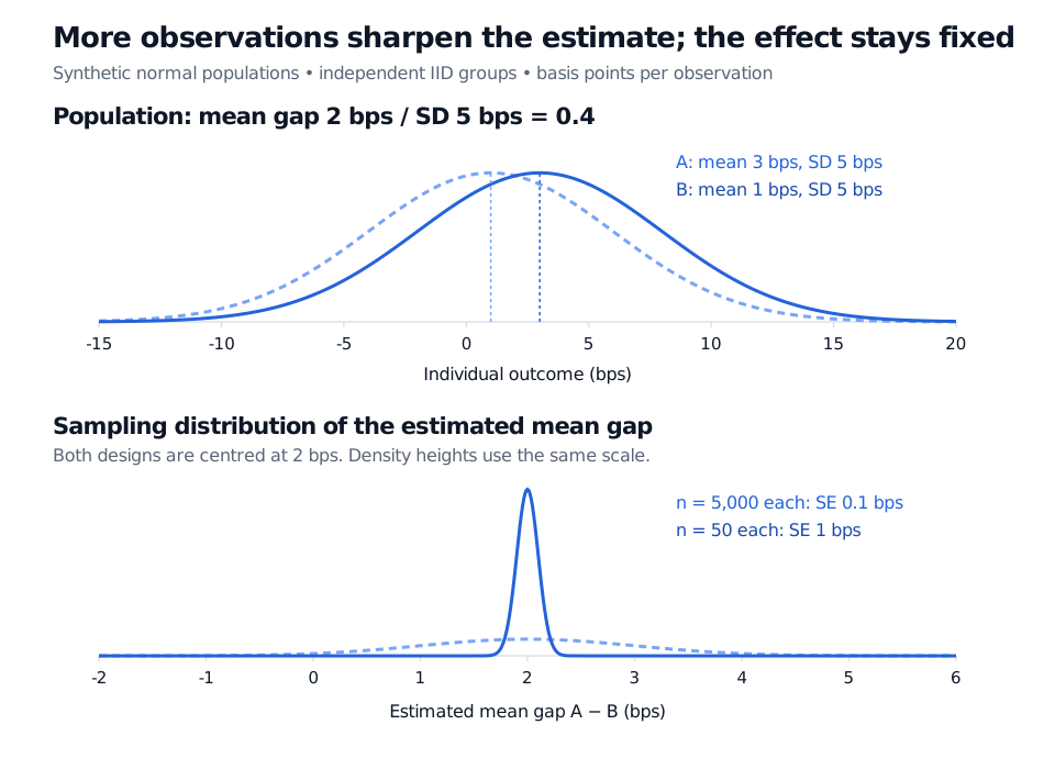
Consider an explicitly synthetic model: independent IID normal observations in each group, also independent across groups. Population means are 3 bps for A and 1 bp for B, with a known common population SD of 5 bps. All quantities refer to one observation; nothing is annualised. Then
Synthetic normal populations A and B have means 3 and 1 bps with common SD 5 bps. Their population mean effect is 2 bps, or 0.4 SD. Sampling distributions of the estimated gap are both centred at 2 bps; their standard deviations are 1 bp at 50 observations per group and 0.1 bps at 5,000.
Original synthetic normal model. Upper panel: individual outcomes. Lower panel: repeated-study estimates, with density heights on a common scale within each panel. Solid blue denotes A above and 5,000 observations per group below; dashed light blue denotes B above and 50 per group below.
Increasing sample size improves precision without changing either population effect. It does not guarantee the same realised estimate in two datasets. Here, under the stipulated alternative, the statistic Z=Δ/SE(Δ) for testing a zero gap has mean 2 in the first design and 20 in the second. Those are means of the statistic's sampling distribution, not observed test results. This is why statistical power can change sharply while effect magnitude stays fixed.
A standardised effect divides by an outcome SD; a test statistic divides by an estimator's SE. Substituting one denominator for the other confuses magnitude with precision. In real return data, dependence and overlapping observations also require a valid uncertainty model; row count alone does not establish this SE.
The denominator is part of the question
Two strategies observed on the same dates often form a paired comparison. With Di=XAi−XBi, one convention is dz=Dˉ/sD, using the SD of the paired differences. Its population analogue uses
σD2=σA2+σB2−2Cov(XA,XB).
That is a different standardiser from the pooled within-group SD. Pairing can change dz through covariance even when marginal means and variances stay fixed. Name the convention and report the raw gap so readers can understand the comparison. An estimated ratio with zero denominator is undefined.
There is no universal economic cutoff for a “large” effect. Two basis points before incremental execution costs may be untradeable; the same raw gain at a different turnover or capacity may matter. Standardisation also cannot make different horizons, risk exposures or data-selection procedures comparable by itself. An observed association or before–after difference does not establish a causal benefit.
Report the effect in useful units, the standardiser if used, and a confidence interval appropriate to the design. For the inference behind those error bars, Confidence Intervals and Hypothesis Testing (membership; public preview) develops normal mean intervals and explains why statistical evidence does not establish trading value.
Larry Wasserman (2004), All of Statistics, Chapter 10, Examples 10.7–10.8, pp. 154–155: independent and paired comparisons and their standard errors. Author's book page.