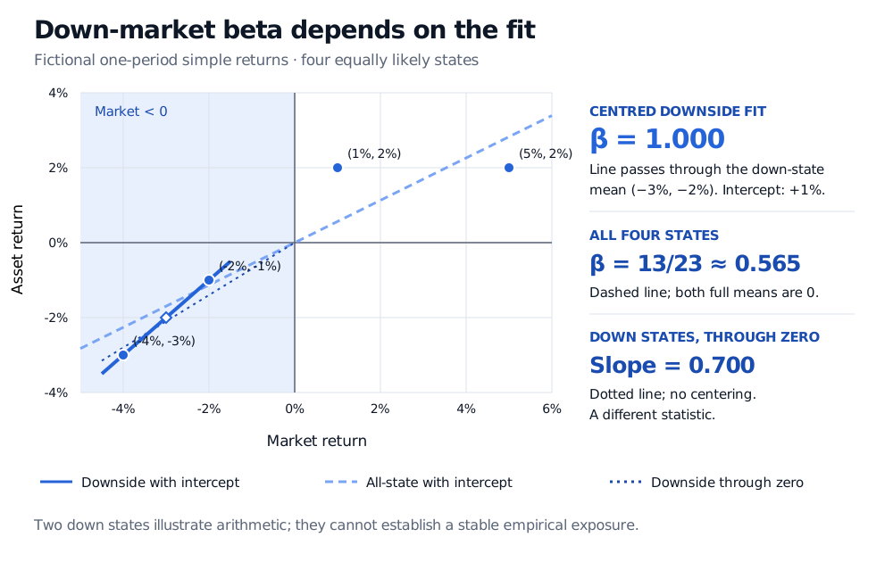
Downside beta measures market sensitivity within a declared down-market region. See why conditional centering gives 1 while a lower-partial ratio gives 0.7.
Downside beta
Downside beta measures an asset’s sensitivity to market returns within a specified down-market region. Under the conditional-covariance convention used here, it is the slope of an asset–market regression with an intercept, using only that region. A manager whose ordinary market beta looks modest may still have substantial exposure when the market falls.
The name alone is insufficient. State which market return counts as “down” and how the observations are centred. Two calculations can select exactly the same bad-market states and still report different betas.
Select the states, then centre within them
Let Ri and Rm be matched-period simple asset and market returns in the same currency. For this article they are raw total returns, not excess returns, and the downside event is D={Rm<0}. With positive event probability, finite conditional second moments and positive conditional market variance, define
βi−(0)=Var(Rm∣Rm<0)Cov(Ri,Rm∣Rm<0).
The covariance and variance are computed around the means within the down-market subset. Write those means as μi,D and μm,D. The numerator is E[(Ri−μi,D)(Rm−μm,D)∣D]; the denominator is E[(Rm−μm,D)2∣D]. Subtracting unconditional means is a different operation.
In historical data, select matched rows satisfying the event and use their own sample means:
This is linear regression fitted on the selected rows with an intercept. The common covariance/variance divisor cancels. No selected observations, or no market variation among them, leaves this beta undefined.
A downside beta of 1 means a one-percentage-point market-return difference corresponds to a one-percentage-point difference along the fitted line within the selected region. The intercept still determines the return level; beta 1 does not say the asset and market have identical losses.
Four states, three answers
Consider this fictional one-period return distribution. Each state has probability 25%; the rows are alternative outcomes, not a price history.
State
Market return
Asset return
Included in D?
A
−4%
−3%
Yes
B
−2%
−1%
Yes
C
1%
2%
No
D
5%
2%
No
Both unconditional means are zero. Conditional on a negative market return, the market mean is −3% and the asset mean is −2%. In decimal-return units, conditional covariance and market variance are both 0.0001, giving
βi−=0.00010.0001=1.
Equivalently, the two down states lie on Ri=0.01+Rm. Moving from market −4% to −2% raises the asset return from −3% to −1%: two percentage points in each series. The intercept is +1%, despite both selected asset returns being negative.
Across all four states, covariance is 0.00065 and market variance is 0.00115. Ordinary beta is therefore
βi=0.001150.00065=2313≈0.565217.
The all-state fit averages over an asset that stops rising between the two positive-market outcomes. It does not describe the slope within the negative-market region.
Four fictional equiprobable states give centred downside beta 1, all-state beta 13/23, approximately 0.565, and down-state through-zero slope 0.7.
Original fictional one-period simple returns. Solid: down-state fit with an intercept. Dashed: all-state fit with an intercept. Dotted: down-state fit through zero. Two down states illustrate arithmetic, not estimation reliability.
Now keep the same negative-market event but calculate an uncentred lower-partial ratio around a zero target:
Here 1 is the event indicator. This is also the slope obtained by fitting the down states through the origin with their probability weights. It retains the products of the negative conditional means; conditional covariance removes them. For example,
E[RiRm∣D]=Cov(Ri,Rm∣D)+μi,Dμm,D.
Thus 1 and 0.7 answer different questions. Neither discrepancy is a rounding error. A provider’s “downside beta” may use a lower-partial construction; inspect its formula before comparing numbers.
The threshold is part of the definition
Ang, Chen and Xing’s Downside Risk, equation (5), uses a conditional covariance slope for excess returns, conditioning on market excess return below its unconditional mean. That is not generally the event “raw market return below zero” or “market excess return below zero.” Their threshold happens to select the same two states in this example if the matched cash return is stipulated to be zero, because the full market mean is zero.
A zero threshold, a cash-return hurdle, a mean-return threshold and a lower-tail quantile can select different observations. Declare strict versus inclusive inequality when a discrete observation can land on the boundary. Subtracting a constant cash return from both series preserves a centred slope for the same selected rows, but changing the threshold can change those rows. A time-varying cash return can change both the slope and selection.
What to take to a risk review
Record the benchmark, currency, return frequency and window, raw or excess basis, threshold, centering rule and number of selected observations. Compare the result with ordinary beta under a consistent return basis. Inspect coefficient uncertainty, influential observations and stability across economically justified windows. Filtering leaves fewer observations; a small conditional market variance makes the ratio especially sensitive to noise.
Our two down states fit two parameters exactly and leave no residual degrees of freedom. The perfect line provides no evidence of a reliably estimated exposure. Ang, Chen and Xing’s Section 3.1 explicitly discusses the need for sufficient downside observations and the trade-off with time-varying exposures; their historical research design is not a universal window prescription.
Downside beta is not maximum drawdown, which requires an ordered wealth path, nor a put’s delta, which is a local derivative of option value. It also differs from a downside capture ratio, which summarises performance relative to a falling benchmark rather than a centred co-movement slope. A low downside beta does not impose a loss floor or establish a future hedge.
For the regression foundations, see Estimating beta in Sharpe’s Single-Index Model. The full lesson requires membership, with a public preview.
Sources
Andrew Ang, Joseph Chen and Yuhang Xing, Downside Risk, author manuscript dated 7 November 2005, equation (5), printed p. 6, and Section 3.1, printed pp. 9–10: conditional excess-return definition, mean threshold and estimation-window considerations. The four-state example, lower-partial comparison and figure here are original calculations.