Deep hedging learns a trading policy under a chosen risk objective, costs and constraints. A cash ledger separates hedge performance from the premium and explains indifference pricing.
Deep hedging
Deep hedging uses deep neural networks to learn a trading policy that manages a derivative liability under a chosen risk objective, trading costs and constraints. The output is a rule for positions as information arrives. This lets a quant optimise the combined liability and trading result when frictionless replication is unavailable or too costly.
The important choice comes before the network: what outcomes count as acceptable, which instruments can be traded, and what each trade costs? A policy trained to reduce severe losses can differ from one trained to minimise squared error. Neither becomes a unique market price merely because a neural network produced it.
Start with the cash, before learning anything
Consider an original synthetic one-step model, in USD per call on one share. Stock starts at 100 and ends at either 90 or 110. A European call has strike 100, so its payoffs are 0 and 10. Interest and dividends are zero; fractional stock holdings and borrowing are allowed.
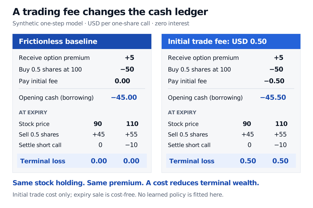
Without frictions, the two payoff equations give a hedge of 0.5 shares and cash of −45. Its opening cost is 5. A writer receiving that premium buys 50 of stock and borrows 45. At expiry the stock is worth 45 or 55; after repaying borrowing, the hedge pays exactly 0 or 10.
Now retain the premium of 5 and the same holding, but charge a stipulated 1% of the initial stock trade's value:
Kinitial=0.01×100×0.5=0.50.
This example charges only the initial trade. The stock is sold cost-free at expiry; there are no intervening trades, funding charges or other fees. The 1% is an arithmetic assumption, not a suggested fee level or a full lifetime trading-cost model.
The opening cash becomes −45.50. In the down state, selling the stock brings in 45 and the option owes nothing: the writer ends at −0.50. In the up state, selling brings in 55, the call costs 10 and the same debt remains: again −0.50.
Synthetic one-step short-call ledger in USD: premium 5 funds half a share bought at 100 with cash minus 45 without costs, or minus 45.50 with an initial fee of 0.50. At terminal stock 90 or 110, losses are zero without costs and 0.50 with the fee.
Original synthetic cash ledger. Same premium and stock holding in both panels; only the initial trade is charged. Expiry sale is cost-free. No neural network is fitted.
Define terminal loss as positive when the writer loses money. For this one-period ledger,
L=C−p−δ(S1−S0)+Kinitial.
Here C is the call payoff, p the premium and δ the share holding. The loss is zero in both states without costs and 0.50 in both with the initial fee. Its variance is zero in either case: zero dispersion alone does not establish an adequate premium. A risk objective must represent the economic question being asked.
The free public sample The Binomial Model derives the stock-and-cash replication baseline. This toy calculation illustrates why adding a cost changes the ledger; it does not establish which policy would be optimal in a larger market.
What the policy learns
At each trading date, a policy takes the information then available—such as current prices, time remaining, relevant history and the previous holding—and outputs a target position. The trade is the change from the old holding to that target. Costs apply to trades, so including the previous position matters.
For several dates and instruments, use discounted monetary units and write terminal loss as
Lθ=C−p−k=0∑n−1δkθ⋅(Sk+1−Sk)+K(δθ).
The network parameters are θ; the dot product adds gains across instruments; K includes the costs specified for the whole strategy, including whatever terminal settlement or liquidation convention is assumed. Position, liquidity and risk limits restrict admissible decisions. Only information available at date k may enter δkθ.
Training searches for parameters that minimise a selected risk measure of this loss, or another explicitly defined loss criterion. An upper-tail expected shortfall objective emphasises bad outcomes; an exponential objective penalises losses according to a risk-aversion parameter. The original paper develops convex risk objectives and neural policy optimisation in §§3–4.
The learned policy need not follow the frictionless delta hedge. Rebalancing can reduce exposure while increasing transaction costs; the objective evaluates their combined effect. It does not guarantee that less trading is always better.
A hedge and a price are separate outputs
A desk can train a policy at a given market premium. Alternatively, it can define an indifference price relative to an optimised no-liability baseline. In a loss convention, let
F(C)=δ∈Ainfρ(C−G(δ)+K(δ)),pind=F(C)−F(0).
Here G is trading gain and A the admissible strategies. Assume the same strategy opportunities in both problems, finite values and a cash-additive loss risk measure: ρ(L−c)=ρ(L)−c. Then receiving pind offsets the incremental optimised risk from taking the claim. The subtraction matters because trading without the liability can itself have value. This is the loss-sign translation of the paper's §3, equation (3.2).
Such a price depends on preferences, dynamics, frictions and constraints. It is not automatically a risk-neutral valuation. In the frictionless attainable-claim case, the paper recovers the replication price under its stated assumptions; that special result should not be carried over to every learned hedge.
What a convincing result must show
A trained network approximates a policy within its inputs, architecture and training scenarios. The paper's approximation result is distinct from finding a global training optimum; §4.3 explicitly notes the lack of a general guarantee of convergence to that optimum in reasonable time.
Assess an actual implementation on unseen paths, with the same starting premium, costs and constraints as its benchmark. Report terminal losses, tail behaviour, turnover, costs and constraint breaches. Changing the premium can improve reported losses without improving the trading policy. The paper's §5.2 comparison explicitly controls this distinction.
Finally, flexibility about the scenario generator is not immunity to model risk. Omitting jumps, understating execution costs or admitting future information into features can make an apparently successful policy fail when traded. Stress scenarios and a reconciled cash account remain essential even when the optimisation runs successfully.
Sources
Hans Buehler, Lukas Gonon, Josef Teichmann and Ben Wood, Deep Hedging, original arXiv manuscript, February 2018. §2, especially equation (2.1), defines self-financed gains, costs and constraints; §3, equations (3.1)–(3.2), Lemma 3.3 and Remark 3.4 separate hedging, indifference pricing and a given premium; §§4.2–4.4 develop neural policies, approximation and optimisation; §§5.1–5.2 describe scenario assumptions and benchmark comparison. The one-step example and figure here are original, not a reproduction of its Heston experiments.