An asset-or-nothing option pays the terminal asset value on a trigger. Distinguish it from a fixed cash digital and see how the two reconstruct a vanilla call.
Asset-or-nothing option
An asset-or-nothing option pays the terminal value of a specified quantity of the underlying asset when a price condition is met, and zero otherwise. Unlike a cash-or-nothing option, its triggered payment varies with the asset price. This makes it a useful building block for separating the asset received from the strike paid in a vanilla option.
Here, the contract is European and cash settled: it pays a cash amount equal to the terminal asset value, rather than delivering the asset. The exposure is one underlying unit, with the asset price and settlement both measured in USD. Other contracts can specify different quantities or delivery terms; the payoff formula alone does not establish those terms.
The trigger decides whether; the asset price decides how much
Write ST for the observed asset price at maturity T and K for the strike price. With a strict trigger, the call and put payments are
ATcall=ST1{ST>K},ATput=ST1{ST<K}.
The indicator function is one when its condition holds and zero otherwise. Under these stated rules, both payments are zero at ST=K. Equality must be specified in the contract: changing > to ≥ changes the payment in that state, even if a continuous pricing model assigns it probability zero.
For a synthetic call struck at USD 100:
Terminal asset price
Asset-or-nothing payment
Vanilla call payment
USD 90
USD 0
USD 0
USD 100
USD 0
USD 0
USD 110
USD 110
USD 10
The strike is only a gate for the asset-or-nothing call: it is not subtracted from the triggered payment. Nor does the last row promise a fixed USD 110 whenever the call triggers. These are terminal payments, before the premium and any funding costs, rather than investment profits.
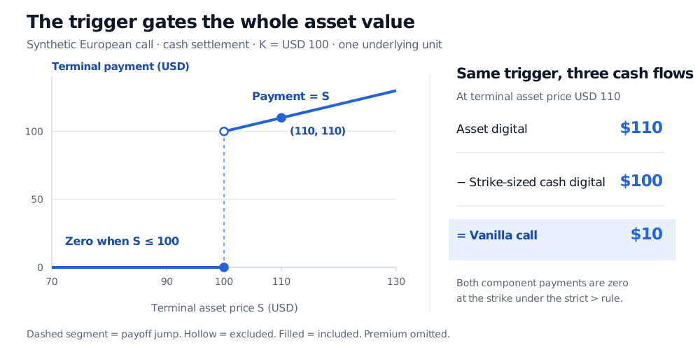
A cash-settled asset-or-nothing call with strike USD 100 pays zero at and below the strike, then pays the terminal asset price above it. At terminal price USD 110 the asset digital pays USD 110, the strike-sized cash digital pays USD 100, and their difference pays USD 10.
Original synthetic payoff diagram for one underlying unit. Hollow points exclude a value; filled points include it. The dashed vertical segment marks the jump, not an attainable series of payments at the strike.
The discontinuity matters: an arbitrarily small move from the strike to just above it switches the call payment from zero to roughly the whole strike amount. Above the threshold, further price increases also increase the payment. The contract therefore combines threshold exposure with asset-price exposure after activation.
Recovering a vanilla call
Let DT=1{ST>K} be a cash digital paying one USD on the same strict trigger. A vanilla call has the exact payoff identity
(ST−K)+=ST1{ST>K}−K1{ST>K}=ATcall−KDT.
At the example’s terminal price of USD 110, the two components pay USD 110 and USD 100, leaving USD 10. Below or at the strike both components pay zero. The same trigger, observation time, quantity and settlement basis are essential to this replication. Mixing an inclusive asset trigger with a strict cash trigger would break it at equality.
By linear pricing, their time-zero values satisfy C0=A0call−KD0 as well. The decomposition is a payoff identity; computing any of those prices requires a valuation framework.
Why its Black–Scholes price uses d1
Under the European Black–Scholes model, with lognormal stock-price dynamics, positive spot, strike, volatility and time to maturity, constant continuously compounded risk-free rate r, and constant continuous dividend yield q,
Here Φ is the standard normal cumulative distribution function and σ is constant volatility. The unit cash call instead has value D0=e−rTΦ(d2).
The distinction is the weighting: the cash digital values the event alone, while the asset digital values ST on that event. High-price states contribute larger cash payments to the asset digital. Consequently Φ(d1) is not the ordinary risk-neutral probability of finishing above the strike; that probability is Φ(d2) under these assumptions.
John C. Hull, Options, Futures, and Other Derivatives, 9th Global Edition, Pearson, 2018, §26.10, p. 629: asset and cash binary prices and the vanilla-option decomposition.