Asset allocation sets the mix of stocks, bonds, cash and other asset classes. Follow a 60/30/10 account through expected return, a loss, weight drift and rebalancing.
Asset allocation
Asset allocation is the choice of how an investment portfolio is divided among asset classes, such as equities, bonds and cash. It sets the broad mix of economic exposures before deciding which securities or funds will deliver them.
A 60% equity allocation is a decision about the share of wealth exposed to equities. Choosing a particular equity fund is a security-selection decision within that share. Two accounts can have identical asset-class weights yet very different concentrations, fees, currency exposures and underlying holdings. Conversely, a single multi-asset fund can implement several asset classes. Count the exposures inside the wrapper, rather than treating every fund as a separate asset class.
A policy, a forecast and an outcome
An allocation can describe either target weights—the intended mix—or current weights, calculated from today's holding values. Keeping those meanings separate prevents an important mistake: a target of 60% equities does not mean equities will remain 60% of the account without trading.
Consider a hypothetical USD 1,000 account invested at the start of one year:
Asset class
Starting value (USD)
Target weight
Assumed one-year expected return
Stocks
600
60%
8%
Bonds
300
30%
3%
Cash
100
10%
1%
These are synthetic assumptions, not observed market estimates or a recommended allocation. Returns are nominal simple total returns in USD over the same year. Income is reinvested within its own asset-class sleeve. There are no contributions, withdrawals or reallocations across asset classes during the year, and no taxes, management fees, transaction charges or bid–ask spreads. Cash is an interest-bearing balance in this example.
Let wi be the starting fraction of wealth in asset class i, and Ri its return over that year. For this fully invested, unlevered account,
That corresponds to expected terminal wealth of USD 1,058 under the assumptions. It is a weighted average of assumed means, not a promised gain of USD 58. The identity does not require the returns to be independent. It also does not tell us the probability of a loss; that needs a model for their joint outcomes.
Now impose a different, realised stress scenario: stocks return −20%, bonds +5% and cash +1%. This is one illustrative outcome, with no probability assigned.
Asset class
Realised return
End-of-year value (USD)
Weight before trading
Stocks
−20%
480
53.57%
Bonds
+5%
315
35.16%
Cash
+1%
101
11.27%
Total
−10.4%
896
100.00%
The account loses USD 104 even though two sleeves gain. The loss on the larger equity sleeve outweighs those gains. The starting weights calculate the realised portfolio return; the end weights describe the resulting account.
More generally, before any end-of-period trade and provided total wealth is positive,
wiend=1+Rpwi(1+Ri).
For stocks, the numerator is their ending value relative to starting wealth; dividing by the account's ending wealth gives 480/896=53.57% after rounding. A falling equity weight here is market drift, not evidence that the investor chose a more defensive policy.
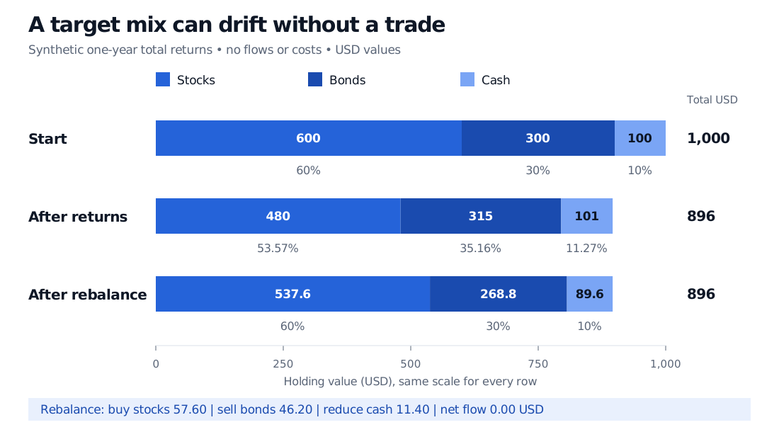
Synthetic USD 1,000 account starts with 600 in stocks, 300 in bonds and 100 in cash. After returns, values are 480, 315 and 101: USD 896 total. Stocks are 53.57% of wealth. Rebalancing restores 60/30/10 with values 537.60, 268.80 and 89.60, leaving total wealth at USD 896.
Original synthetic one-year example. Bars use a common USD scale; percentages describe each row's own total. No external flows or costs. Restoring the mix leaves the loss intact.
What a rebalance actually changes
To restore the original mix, apply 60/30/10 to USD 896, not to the original USD 1,000. Assume trades occur immediately after the year-end valuation at those same marks, with fractional holdings permitted and no costs.
Asset class
Before trade (USD)
Restored target value (USD)
Trade in value (USD)
Stocks
480.00
537.60
+57.60
Bonds
315.00
268.80
−46.20
Cash
101.00
89.60
−11.40
Total
896.00
896.00
0.00
A positive trade buys exposure; a negative trade sells or reduces it. Bond sales fund USD 46.20 of the equity purchase and reducing cash funds the remaining USD 11.40. The ledger is self-financing. Rebalancing changes future exposure; it creates no immediate profit in this frictionless example and does not guarantee a better subsequent return.
An actual policy needs a trigger: perhaps a calendar review or a specified deviation from target weights. Contributions can also be directed to underweight classes. Costs and taxes can make exact restoration undesirable, so a tolerance band can be more practical than continuous trading. The SEC's allocation guide explains these implementation choices. With external cash flows, update the investable wealth and cash-flow timing explicitly before calculating trades or measuring performance.
Choosing the mix is a risk decision
A strategic allocation sets a longer-term policy mix. A tactical allocation deliberately departs from it based on shorter-term views. Neither is the same as accidental drift. A scheduled review may also change the policy itself as spending needs or circumstances change; that is different from trading back to an unchanged target.
Useful inputs include when money must be available, the size and flexibility of future spending, tolerance and capacity for losses, and restrictions on liquidity, leverage or eligible investments. The SEC's introduction connects the allocation decision to time horizon and risk tolerance. A long horizon does not make risky assets certain to recover before a particular payment date.
Asset-class labels alone are too coarse to measure risk. Long-duration government bonds and short-term bills have different rate sensitivity; lower-quality corporate bonds can carry substantial credit exposure. Foreign assets can add currency risk. Cash can be stable in nominal account units while losing purchasing power through inflation.
Diversification depends on how the underlying exposures move together, not just the number of rows in an allocation table. Portfolio variance depends on weights and covariance; 60% of capital in an asset class need not mean 60% of portfolio risk. Stock and bond returns can both be negative. The positive bond return in our stress example is an assumption, not a rule about what bonds do in an equity sell-off.
Mean–variance optimisation formalises one way to choose weights using expected returns, covariances and constraints. It remains conditional on those inputs and the chosen objective. For the mathematical next step, Mean-Variance Optimisation develops the portfolio moment formulas and allocation problems with and without cash. Its full lesson requires membership; a public preview is available.
Sources
Elton, E. J., Gruber, M. J., Brown, S. J. and Goetzmann, W. N. Modern Portfolio Theory and Investment Analysis, 9th edition, Wiley, 2014. Chapter 10, “Estimating Expected Returns,” pp. 206–208, especially “Aggregate Asset Allocation” and “Market Timing or Dynamic Asset Allocation.”