The X-learner estimates a conditional average treatment effect by imputing missing outcomes, fitting effect regressions separately in the treated and control groups, and blending their predictions. In an execution experiment with many orders using the incumbent rule and few using a new rule, it offers a way to use the large control sample to help estimate how the new rule's benefit varies across order characteristics. It is a recipe for combining regression models, rather than one particular model family.
Cross the predictions, then learn the effect
Let denote treatment, control, pre-treatment features and the observed outcome. First fit two outcome regressions: using control observations, and using treated observations. Construct the pseudo-outcomes
Each observed outcome is paired with the other group's outcome prediction. Both differences use the treatment-minus-control sign. Next regress the treated pseudo-outcomes on their features to obtain , and the control pseudo-outcomes on their features to obtain . The subscripts identify the group supplying the second-stage observations, not two different causal targets.
The final prediction is
This follows Künzel et al., X-Learner, equations 5–9 and Remark 1. Here weights the control-group effect regression. An estimated propensity score, , is a suggested choice for , not a mandatory or universally optimal weight.
Two imputed differences are not a fitted effect surface
Consider fictional execution benefits in basis points per order, relative to a fixed benchmark and after consistently measured costs; higher is better. Treatment means switching to the new execution rule. The numbers below are stipulated observations and predictions, with no uncertainty estimates supplied.
| Observation | Observed outcome | Prediction under the other rule | Imputed effect |
|---|---|---|---|
| Treated order | 7 bp | Control: 3 bp | bp |
| Control order | 2 bp | Treatment: 6 bp | bp |
These are noisy training labels, not observed individual causal effects. A prediction of what the first order would have earned under control does not reveal its missing potential outcome.
Separately, suppose second-stage models trained on a larger dataset predict bp and bp at a chosen feature value. These predictions are stipulated; they are not fits from the two rows above. With ,
The result lies between the two predictions and is closer to 4 bp because that prediction receives three-quarters of the weight. Reversing which model gets would answer a different calculation.
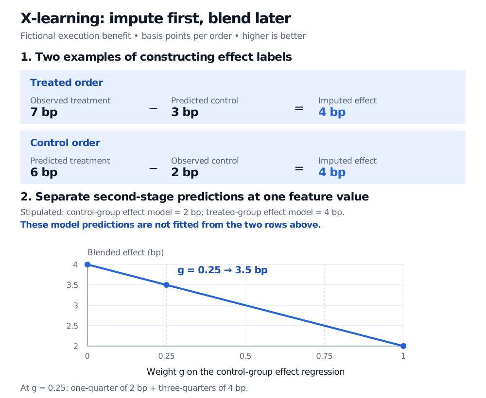
Original fictional illustration. Top: two imputation examples. Bottom: separately stipulated effect-model predictions at one feature value, not fits from those two observations. The blend uses weight g on the control-group effect regression.
Why imbalance can help—and where it cannot
A large control sample can support a good control-outcome fit. Subtracting that fit from treated outcomes can leave an effect function simpler than either outcome surface. When treatment is rare locally and , the blend emphasises : the treated-group effect regression whose labels use the control-outcome model. The reverse logic applies with abundant treated observations. These are advantages under suitable structure and estimation quality, not an automatic benefit from imbalance. Künzel et al., Intuition Behind the Metalearners give the mechanism.
Imbalance also differs from absent causal overlap. For causal interpretation, the baseline setup requires well-defined actions and consistency, no unaccounted interference, conditional exchangeability of potential outcomes and assignment given , and both assignments possible at the features being studied. Under those conditions,
Nie and Wager, §2 state the potential-outcome and exchangeability setup; Kennedy, §2 lists consistency, positivity and no unmeasured confounding. If an unrecorded urgency signal drives both execution-rule choice and outcomes, the regressions do not establish comparability. If a feature region contains only control orders by design, more control observations do not identify treatment response there. A fitted curve can still extrapolate into that region.
Separate it from S-, T-, R- and DR-learning
An S-learner uses one outcome model with treatment as a feature and contrasts its two treatment settings. A T-learner subtracts two separately fitted outcome predictions. The X-learner adds effect-label regression and blending. Nie and Wager, §6.1 describe these baselines.
An R-learner instead fits an effect function through a loss relating outcome residuals to treatment residuals. A DR-learner regresses an augmented inverse-probability-weighted pseudo-outcome on features. A propensity-weighted X-learner blend does not confer the latter's double robustness: combines effect predictions; it does not supply the DR pseudo-outcome's inverse-probability residual correction. See Nie and Wager, §§2–3 and 5 and Kennedy, §§4.1–4.2.
For flexible models, separate nuisance fitting, tuning and final evaluation. Cross-fitting can keep a held-out fold's outcomes out of the models used to construct its pseudo-outcomes; it does not change the X-learner into an orthogonal or doubly robust procedure. Second-stage predictions also need independent evaluation, with time and dependence respected for financial data. No individual causal label becomes available merely by holding an observation out.
Conditional Expectation (membership; public preview) explains the averaging foundation: regression targets a conditional mean of noisy labels. It does not make each label an individual counterfactual.
Sources
- Künzel, Sekhon, Bickel and Yu (2019), Metalearners for estimating heterogeneous treatment effects using machine learning. PNAS article, X-Learner, equations 5–9; Remark 1; Intuition Behind the Metalearners.
- Nie and Wager, Quasi-Oracle Estimation of Heterogeneous Treatment Effects. Primary manuscript, §§2–3, 5 and 6.1.
- Kennedy, Towards Optimal Doubly Robust Estimation of Heterogeneous Causal Effects. Primary manuscript, §§2 and 4.1–4.2.