Conditional average treatment effect and uplift modelling
Conditional average treatment effects describe how an intervention changes outcomes across features. Learn the uplift target, causal assumptions and population averaging.
Conditional average treatment effect and uplift modelling
The conditional average treatment effect (CATE) is the expected change in an outcome caused by an intervention, among units with specified observed features. Uplift modelling estimates this incremental effect to help decide where an action is useful. For a quant comparing execution rules, a positive effect across all orders can conceal a subgroup for which switching rules makes execution worse. The target is the difference the switch makes, rather than the outcome a rule happens to predict. Gutierrez and Gérardy, §§2–3 connect uplift modelling to this causal target.
Average for whom, under which action?
Let W=1 mean using a new execution rule and W=0 mean using the existing rule. In the potential outcomes framework, Y(1) and Y(0) are the outcome under each action. Let X contain features recorded before assignment, such as the order's initial size and the prevailing spread. Then
τ(x)=E[Y(1)−Y(0)∣X=x].
The expectation averages over units sharing the features x. More detailed features can change this average; “conditional” does not mean that every relevant individual characteristic is known. With continuous features, estimation typically borrows information from nearby or otherwise similar feature values.
For an individual order, the treatment effect is Y(1)−Y(0). Only the outcome under its assigned action is observed: Y=Y(W). A fitted CATE for that order's features therefore does not reveal its missing individual counterfactual. Even a perfectly known subgroup average can contain both helped and harmed orders. Künzel et al., Framework and Definitions distinguish these targets.
A positive average can hide a harmful switch
Consider a fictional population in which the causal conditional means below are stipulated as known. The outcome is net execution benefit relative to a fixed arrival-price benchmark, in basis points per order; higher is better. Costs of the two rules are included consistently. Groups A and B are defined before treatment and exhaust the target population.
Pre-treatment group
Population share
Mean benefit under existing rule
Mean benefit under new rule
CATE: new minus existing
A
75%
1 bp
3 bp
+2 bp
B
25%
4 bp
3 bp
−1 bp
Both groups have the same mean outcome under the new rule. Their incremental effects nevertheless have opposite signs because their alternatives differ. Predicting who will perform well under treatment alone would miss this distinction.
The average treatment effect averages the conditional effects using the target population's feature distribution:
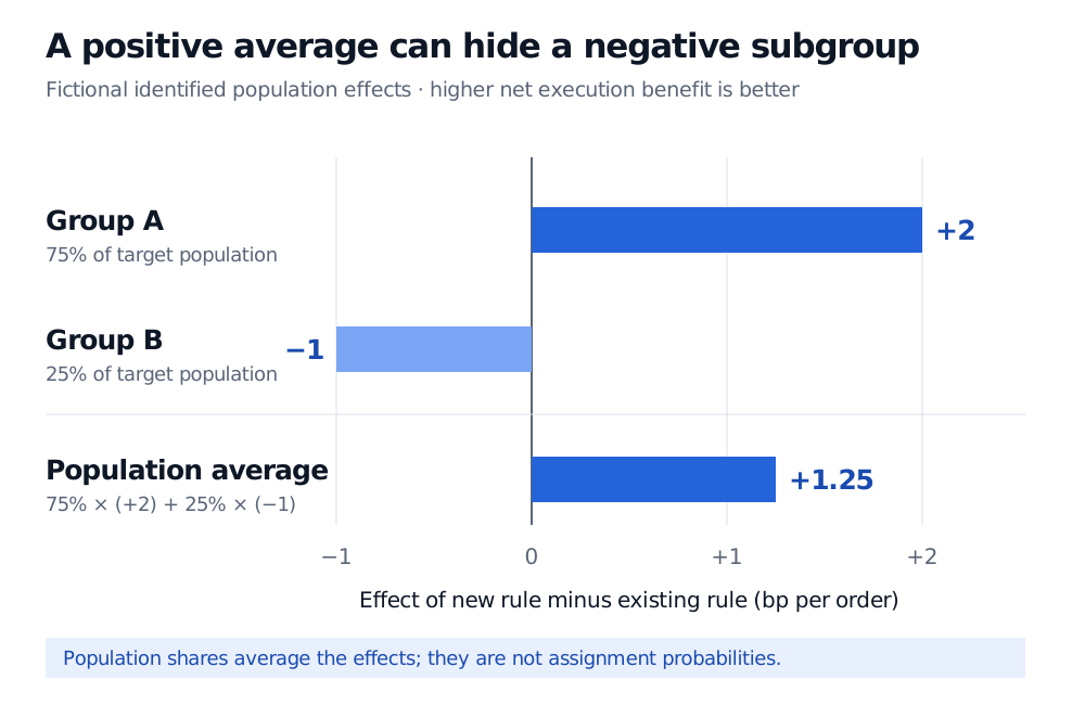
ATE=E[τ(X)]=0.75(2)+0.25(−1)=1.25bp.
The unconditional potential-outcome means give the same result: the new rule yields 3 bp on average, compared with 1.75 bp under the existing rule. The weights are population shares, not treatment-assignment probabilities.
Fictional population conditional effects: group A, 75 percent of orders, gains 2 basis points; group B, 25 percent, loses 1 basis point. Their weighted average treatment effect is plus 1.25 basis points per order.
Original fictional population example. The positive average does not remove the negative effect in group B. These are stipulated causal means, not fitted estimates or realised returns.
Under these exact means, switching A while retaining the existing rule for B improves the population mean by 1.5 bp, versus 1.25 bp from switching everyone. That calculation assumes the outcome already captures relevant costs, both choices are feasible, and selective deployment does not change anyone else's outcomes. Capacity limits, market impact or changes in the order mix can invalidate that comparison. No sample size or uncertainty estimate is supplied.
Conditional Expectation (membership; public preview) develops the averaging rule behind the CATE-to-ATE calculation and separates a conditional mean from an individual realisation.
When observed differences identify the effect
A treated-versus-control outcome gap within features is observable in principle. Giving it a causal interpretation needs a design. In the baseline binary-action setting, sufficient conditions include:
Consistency and well-defined actions: an order assigned a specified rule has the potential outcome for that rule. “New algorithm” must identify an intervention precisely enough to compare its versions.
Conditional exchangeability:(Y(1),Y(0))⊥W∣X. Assignment carries no remaining information about potential outcomes once the relevant pre-treatment features are held fixed. Suitable randomisation supplies this comparability by design; an observational study must justify it.
Positivity:0<P(W=1∣X=x)<1 at the feature values being studied. Both actions must be possible.
No unaccounted interference: one order's assignment must not change another order's outcome within this simple potential-outcome specification.
Under these conditions,
τ(x)=E[Y∣W=1,X=x]−E[Y∣W=0,X=x].
Künzel et al., Framework and Definitions state the comparability and overlap conditions; Athey and Wager, §1.1 illustrate why selection and clustered observations matter. An unrecorded urgency signal could drive both rule choice and execution quality. Accurate outcome prediction would not remove that confounding. Conditioning on a fill rate measured after assignment can also change the causal question rather than repair it.
Estimating uplift without pretending to observe it
A T-learner fits separate outcome models in the treated and control groups, then subtracts their predictions at the same features. An S-learner fits one outcome model including the treatment indicator and compares its predictions under the two indicator values. Causal trees and causal forests instead adapt partitions or ensembles to effect heterogeneity. These are estimation choices; none establishes the identifying assumptions. Künzel et al., Meta-algorithms explain the first two constructions.
Ordinary prediction accuracy is an incomplete evaluation: no observed individual-effect label exists against which to score each prediction. Held-out treated/control comparisons within predeclared score groups can assess average effects when the design and adjustment justify them. Selecting the groups on those same outcomes risks discovering noise. Gutierrez and Gérardy, §4 discuss uplift evaluation under this missing-counterfactual constraint.
For financial deployment, assess the resulting decision rule on information available at decision time, with uncertainty and market dependence accounted for. A model that estimates heterogeneous means does not by itself establish a stable, economically valuable allocation rule in a changed market.
Sources
Künzel, Sekhon, Bickel and Yu (2019), Meta-learners for Estimating Heterogeneous Treatment Effects using Machine Learning, Framework and Definitions; Meta-algorithms. Primary manuscript.
Gutierrez and Gérardy (2017), Causal Inference and Uplift Modelling: A Review of the Literature, §§2–4. PMLR paper.
Athey and Wager (2019), Estimating Treatment Effects with Causal Forests: An Application, §1.1. Primary manuscript.