Separate the outcome forecast from a heterogeneous treatment effect, fit cross-fitted residuals with R-loss, and see how overlap and regularisation change the problem.
R-learner and Robinson decomposition
The R-learner estimates a treatment-effect function by fitting the relationship between residualised outcomes and residualised treatment assignments. The Robinson decomposition is the population identity behind that fit. For a quant comparing two execution policies, it separates predictable cost differences associated with order characteristics from the cost change attributed to the policy, under explicit causal assumptions.
The target is a conditional average treatment effect, not a prediction of the observed outcome and not an individual order's unobserved counterfactual.
Remove the outcome mean, not the untreated baseline
Let D∈{0,1} identify the policy, Y denote execution cost in basis points, and X contain pre-treatment order characteristics. Define
Thus m(x) is the observed outcome mean mixing both policies. It is not the untreated response μ0(x). Subtracting it from Y=μ0(X)+Dτ(X)+ε, where E[ε∣X,D]=0, gives
Y−m(X)={D−e(X)}τ(X)+ε.
Nie and Wager, §2, use this Robinson residualisation identity to construct the R-learner. Robinson's original setting estimated a constant coefficient in a partially linear model; here the coefficient can vary with X.
The algebra describes conditional observed means. Its causal interpretation additionally needs consistent potential outcomes, a well-defined treatment without interference, no unmeasured confounding conditional on X, and overlap. Residualisation cannot establish those assumptions. In the execution example, policy choices based on unrecorded urgency could invalidate the causal interpretation.
Fit residuals with an effect-specific loss
Use cross-fitting to obtain each row's nuisance predictions from models trained outside its fold. Write
ri=Yi−m^(−k(i))(Xi),di=Di−e^(−k(i))(Xi).
Then minimise the R-loss, with a complexity penalty on the candidate effect function g:
τ^∈gargmin{n1i=1∑n{ri−dig(Xi)}2+Λ(g)}.
This is a loss framework, not a particular tree or neural network. A constant g(x)=t fits one effect; a richer class can learn heterogeneity. Out-of-fold nuisance fitting prevents each row from helping construct its own nuisance prediction. It does not by itself supply a valid dependence model for repeated orders, firms or trading days.
For the unpenalised constant fit, differentiation gives
t^=∑idi2∑idiri,i∑di2>0.
This is a slope through the origin in residual space, not generally the raw difference between treated and untreated outcome means.
Two rows reveal the mechanics
Suppose held-out nuisance predictions produce the following fictional residuals. These are stipulated inputs, not an estimated causal study.
Row
Treatment residual di
Cost residual ri (bps)
A
−0.5
−1
B
0.5
1
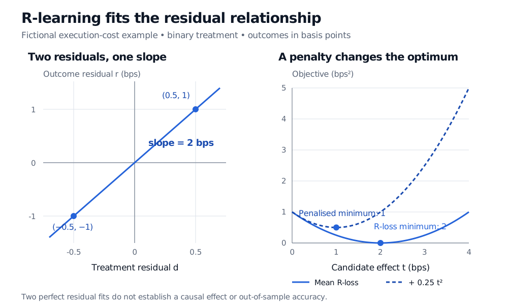
The cross-product sum is 1, and the squared treatment-residual sum is 0.5. The fitted constant is therefore 2 bps, with both residual errors exactly zero. A positive effect means higher execution cost under policy 1 under the stated sign convention.
For these two rows the mean R-loss is 41(t−2)2. If we deliberately add the penalty Λ(t)=41t2, the objective becomes
41(t−2)2+41t2=21(t−1)2+21.
Its minimum is now t=1 bps. The unpenalised R-loss there is 0.25 bps squared, and the total objective is 0.5 bps squared. Penalty choice changes the answer even though the nuisance residuals are unchanged. Neither fit establishes generalisation from two observations.
Fictional cost residuals minus 1 and 1 bps against treatment residuals minus 0.5 and 0.5 lie on a line of slope 2 bps. Mean R-loss is zero at effect 2. Adding a penalty of 0.25 times the squared effect moves the minimum to effect 1, with penalised objective 0.5 bps squared.
Original two-row residual calculation. The right panel uses mean R-loss and a specified quadratic penalty; the dashed curve includes the penalty.
What low R-loss can hide
With the true nuisances and finite second moments, expand the squared residual and use the zero conditional mean of ε. The excess population R-loss for a candidate g is
L(g)−L(τ)=E[e(X){1−e(X)}{g(X)−τ(X)}2].
This identity exposes the weighting: errors where assignment is nearly deterministic contribute little to the loss. With no overlap, some effects are unidentified; with weak overlap, a low aggregate loss can coexist with poor effect estimates in those regions. Restricting the function class or adding a penalty also trades fit against complexity, so the fitted effect need not equal the unrestricted population target.
The local nuisance-error protection is related to Neyman orthogonality. It does not promise accurate effects from arbitrary nuisance models. Nie and Wager's quasi-oracle theorem concerns a specific penalised kernel learner under overlap, nuisance-rate and uniform-consistency conditions, boundedness and kernel/smoothness restrictions, and a suitable penalty. It is not a universal oracle guarantee for any R-learner implementation; see §5, Theorem 3.
For the residual's mean-zero foundation, the owned Conditional Expectation lesson develops the tower property and squared-error projection. Its preview is public; the full lesson requires membership.