A score can be locally insensitive to nuisance-model error. Derive that protection, calculate its quadratic remainder, and see what it leaves unresolved.
Neyman orthogonality
Neyman orthogonality is a local property of an estimating score: at the true target and nuisance values, the derivative of its population expectation with respect to admissible nuisance perturbations is zero. A nuisance is an auxiliary quantity, such as a conditional mean, needed to estimate the parameter of interest. For a quant estimating an execution-policy coefficient after learning market-condition effects, orthogonality can prevent small nuisance errors from entering the estimating equation at first order.
The protection belongs to a particular score and parameterisation. It is neither a statement that two data vectors meet at a right angle nor a guarantee that arbitrary machine-learning predictions yield valid inference.
Which derivative vanishes?
Let W denote observed data, θ0 the true target, η0 the true nuisance object and ψ the score. Start with the valid population moment
E[ψ(W;θ0,η0)]=0.
For an admissible direction h, take a path ηr=η0+rh that stays within the nuisance space near zero. Orthogonality requires the Gateaux, or pathwise, derivative
drdE[ψ(W;θ0,η0+rh)]r=0=0
for all directions in the specified nuisance deviation set, with the derivative existing. The data distribution and θ0 stay fixed. This is a derivative of the expected score; individual observations' scores need not have zero derivatives. Chernozhukov and coauthors' Definition 2.1 makes the deviation set explicit.
Residualising both sides
Consider the partially linear model
Y=θ0D+a0(X)+U,E[U∣D,X]=0.
Here Y is an outcome, D a policy variable and X observed controls. Define the conditional means
g0(X)=E[Y∣X],m0(X)=E[D∣X].
Crucially, g0=θ0m0+a0: the outcome mean g0 is not the structural function a0. We use g for the outcome mean; the original paper calls it ℓ in its partialling-out score, equation (4.4).
With V=D−m0(X), subtraction gives Y−g0(X)=θ0V+U. Use
ψ(W;θ,g,m)={Y−g(X)−θ[D−m(X)]}[D−m(X)].
At the truth this is UV, with expectation zero. To see the local protection directly, perturb g0 by rhg and m0 by rhm. Expanding the two factors gives
All direction functions here are evaluated at X. Assume the products are integrable, for example with square-integrable residuals and directions. The linear terms vanish because E[V∣X]=0 and E[U∣X]=0. The remaining expression has zero derivative at r=0.
The Conditional Expectation lesson develops these residual and tower-property identities. The public page previews the lesson; full teaching requires membership.
A two-state population you can audit
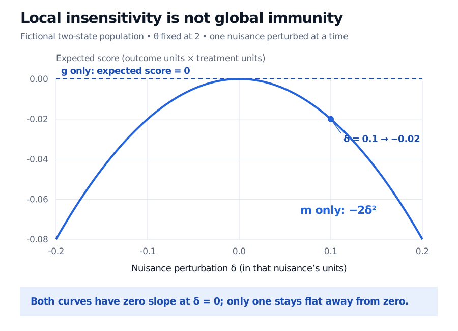
Take a fictional population with no varying controls and two equally probable states. Let (D,Y) be (0,1) or (1,3). Then m0=0.5, g0=2 and θ0=2; the structural intercept is a0=1 and U=0.
Hold θ=2 fixed while changing one nuisance at a time:
Nuisance values
Score when D=0
Score when D=1
Expected score
g=2,m=0.5
0
0
0
g=2.1,m=0.5
0.05
−0.05
0
g=2,m=0.6
−0.12
0.08
−0.02
For the last row the outcome residuals inside braces are both 0.2, while the treatment residuals are −0.6 and 0.4. Their products average to (−0.12+0.08)/2=−0.02. In general, changing only m by δ gives −2δ2: no linear term, but a nonzero quadratic error.
In a fictional balanced two-state population, changing the outcome mean g alone leaves the expected score zero. Changing the treatment mean m by delta gives minus 2 delta squared, reaching minus 0.02 at delta 0.1; both curves have zero slope at delta zero.
Original population sensitivity calculation at fixed theta equal to 2. Zero slope at the truth does not mean zero error away from it.
This is an exact finite population calculation, not a two-observation proof of asymptotic normality. Its zero outcome noise also rules out using it to illustrate a nondegenerate sampling variance.
Local protection still needs an estimation design
For fixed nuisance errors Δg=g−g0 and Δm=m−m0, the expansion above gives the exact moment error
E[ψ(W;θ0,g,m)]=E[ΔgΔm]−θ0E[(Δm)2].
This also shows why orthogonality does not automatically mean double robustness. Setting Δg=0 leaves the squared treatment-mean error. One correct nuisance is not sufficient in either direction for this parameterisation.
In double machine learning, cross-fitting controls the use of each observation in nuisance fitting; orthogonality controls population sensitivity. The author introduction, §§2.3.1–2.3.2, explains their distinct roles. A zero population derivative does not remove same-sample overfitting terms.
For this partialling-out score, an important nuisance-rate condition is
∥m−m0∥2(∥g−g0∥2+∥m−m0∥2)=op(n−1/2),
where ∥f∥2=(E[f(X)2])1/2. It is not the whole theorem. The original paper's Assumption 4.1 and Theorem 4.1 also impose sampling, moment, nuisance-consistency and nondegeneracy conditions. In particular, E[V2] must stay away from zero: the target coefficient cannot be learned from treatment residuals with no variation. Dependent financial observations need an appropriate splitting and inference theory.
Finally, causal interpretation requires identification assumptions. Residualising observed controls does not remove unobserved confounding or create overlap. Orthogonality protects an estimating equation locally after its target and model have been justified.