Compare one pooled outcome model with two policy-specific models for conditional treatment effects, including interactions, shrinkage, imbalance and causal overlap.
S-learner and T-learner
An S-learner estimates a treatment effect by fitting one outcome model with treatment assignment included as a feature. A T-learner fits separate outcome models for the treated and control groups. Both subtract predictions at the same features to estimate the conditional average treatment effect, or CATE. For a quant comparing execution policies, the choice determines how information is shared between policies—and which differences the model can express.
Same target, different use of the data
Let D=1 denote the new execution policy and D=0 the existing policy. Let X contain features available before policy assignment, and let Y be execution cost in basis points, measured over the same horizon and benchmark for both policies. A positive effect means the new policy raises cost.
The causal target, expressed using potential outcomes, is
τ(x)=E[Y(1)−Y(0)∣X=x].
The two constructions are:
Architecture
Fit
Predict the contrast at the same x
S: single model
Fit m(x,d) to all observations, including D as a predictor
τS(x)=m(x,1)−m(x,0)
T: two models
Fit m1(x) using only D=1 observations and m0(x) using only D=0 observations
τT(x)=m1(x)−m0(x)
The base learner can be a regression, forest or another suitable outcome predictor. “S” and “T” describe the arrangement, not a particular learning algorithm. The official EconML descriptions of its S-learner and T-learner implement this distinction.
A subtraction you can audit
Consider fictional, stipulated prediction functions. No data have been fitted. Take a scalar pretreatment feature value x=4; its scale is arbitrary, while predictions are in basis points.
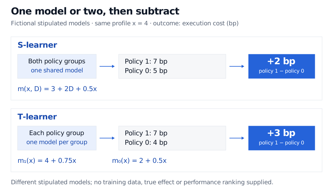
For the S-learner, suppose
m(x,d)=3+2d+0.5x.
At x=4, changing the indicator from 0 to 1 gives predictions of 5 bp and 7 bp. The estimated effect is 7−5=2 bp. The feature contribution cancels, so this particular model imposes a constant effect of 2 bp at every x.
For the T-learner, instead stipulate
m1(x)=4+0.75x,m0(x)=2+0.5x.
The same profile gives 7 bp under policy 1 and 4 bp under policy 0: an estimated effect of 7−4=3 bp. Here the contrast is 2+0.25x.
Fictional stipulated models at x equals 4: one S model predicts 7 and 5 basis points, giving plus 2; separate T models predict 7 and 4 basis points, giving plus 3. Both use policy 1 minus policy 0.
Original architecture diagram with stipulated execution-cost predictions. The difference between 2 bp and 3 bp is not evidence that either learner is more accurate.
The different answers arise from different supplied functions. There is no true effect or test sample here with which to choose a winner.
Nor is an S-learner inherently restricted to constant effects. The single function
m(x,d)=2+0.5x+d(2+0.25x)
reproduces both stipulated T-model surfaces exactly. Its treatment–feature interaction permits the slope to change with policy. This algebra concerns representation; it does not imply that fitting or penalising the two parameterisations produces the same estimates.
Sharing information can help—or suppress the contrast
With an S-learner, regularisation or a tree's split selection may ignore treatment and its interactions. Predictions under both policies then coincide, producing zero estimated effect. That can help when effects are absent, or hide a real effect. A T-learner permits separate shapes but does not automatically share common structure across arms. If one group is small, its surface can be poorly estimated even when the other group is large. These trade-offs depend on the base learner and data; Künzel et al., Simulation Results demonstrate that there is no uniformly best choice.
Ridge, Lasso, and Elastic Net explains coefficient shrinkage and variable selection—the mechanism behind the penalised-regression version of this concern. Its public page is a preview; the full lesson requires membership.
Treatment-group imbalance is also different from missing local overlap. Both policies must be possible at the profiles being compared. Having many control orders does not supply treated outcomes for a profile never treated. The X-learner adds effect-regression stages to exploit structure and imbalance; it cannot manufacture identification. Künzel et al.'s Framework and Definitions and X-learner sections separate these issues.
Prediction is only one part of a causal comparison
To interpret the fitted contrast causally, assignment must be comparable conditional on the chosen pretreatment features: (Y(1),Y(0))⊥D∣X. The policies must be well defined, with consistency requiring the observed outcome to match the specified policy's potential outcome, Y=Y(D). Gutierrez and Gérardy, §2 explain this distinction between an observed conditional gap and a causal effect. An unrecorded urgency signal that drives both policy choice and cost creates confounding that neither architecture removes. The unit-level comparison also assumes no unaccounted interference: one order's policy must not alter another order's cost. Competing orders can violate that assumption, requiring a causal model that specifies spillovers. Halloran's account of interference explains why assignment to other units can change the target.
Finally, outcome-prediction accuracy does not directly measure effect accuracy: each order reveals only one policy outcome, not its individual causal difference. A sound comparison needs held-out causal evaluation justified by the assignment design, rather than choosing whichever model has the lowest ordinary outcome error. Gutierrez and Gérardy's §§3.1 and 4 explain the weaker effect signal and evaluation problem.
Sources
Künzel, Sekhon, Bickel and Yu (2019), Meta-learners for Estimating Heterogeneous Treatment Effects using Machine Learning. Original manuscript, Framework and Definitions, Meta-algorithms, X-learner and Simulation Results.
PyWhy, EconML 0.16.0 documentation: SLearner and TLearner, class descriptions and estimator parameters.
Gutierrez and Gérardy (2017), Causal Inference and Uplift Modelling: A Review of the Literature. PMLR paper, §§2, 3.1 and 4.
Halloran, Towards Causal Inference with Interference, University of Washington seminar abstract describing Hudgens and Halloran (2008). Author presentation summary.