Here is the policy used, contains pretreatment characteristics, and is the outcome under policy . For execution cost measured in basis points, a positive effect means policy 1 raises cost relative to policy 0. Specify the execution rules, horizon and treatment of unfilled orders before estimating this quantity.
Build a response, then learn its conditional mean
Let and let be the [propensity score. Fit estimates of these nuisance functions on a separate training sample. For an observation excluded from that fit, construct
The regression learns the effect function directly, which can be simpler than either outcome surface. It does not treat each pseudo-outcome as an observed individual causal effect.
One row gives 4; the conditional effect can be 2
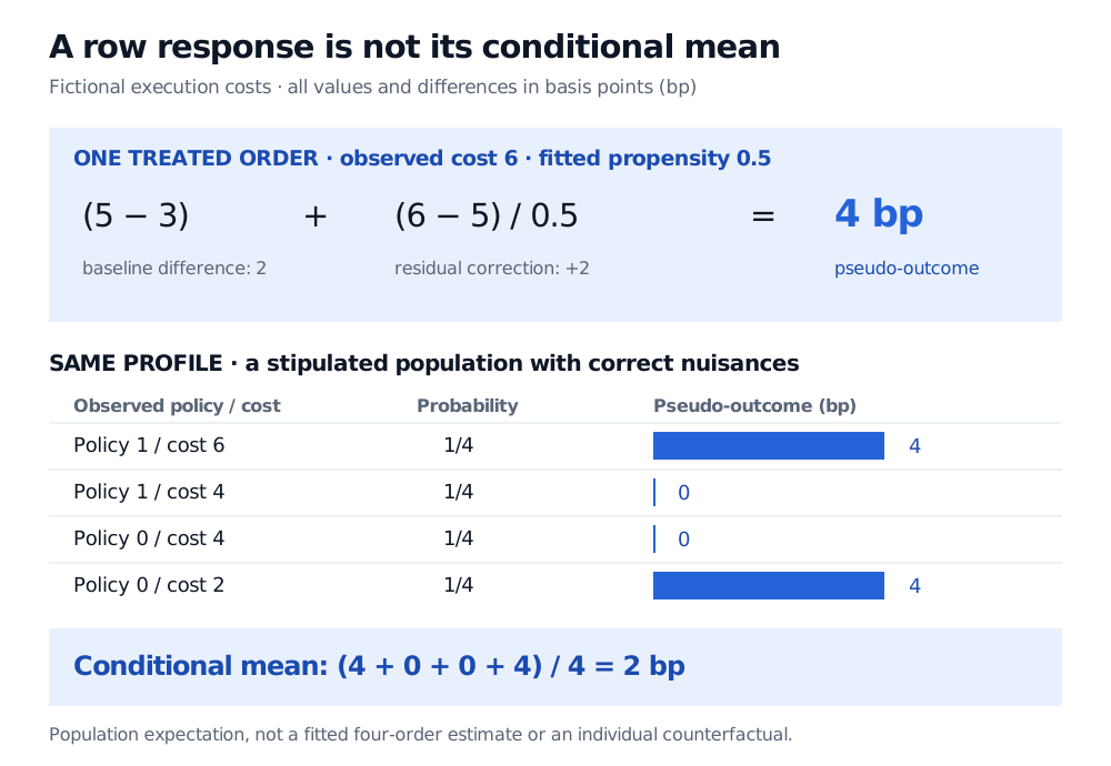
Consider a fictional order profile. Suppose the nuisance predictions are , basis points and . An order receives policy 1 and its observed cost is 6 basis points. Its pseudo-outcome is
The untreated correction is zero because this order received policy 1. We have not observed what its cost would have been under policy 0. If that unobserved cost were 4, its individual effect would be 2, despite the pseudo-outcome of 4.
To see what the second stage targets, stipulate a complete fictional population at this same profile: policy assignment is independent with probability one half; policy-1 costs are equally likely to be 4 or 6, and policy-0 costs equally likely to be 2 or 4. The two potential costs are independent. The true conditional means are therefore 5 and 3, and the CATE is 2 basis points. Using those correct nuisances gives:
| Observed policy | Observed cost (bp) | Population probability | Pseudo-outcome (bp) |
|---|---|---|---|
| 1 | 6 | 1/4 | 4 |
| 1 | 4 | 1/4 | 0 |
| 0 | 4 | 1/4 | 0 |
| 0 | 2 | 1/4 | 4 |
Thus the pseudo-outcome's conditional mean is . This is a population calculation, not a fitted four-observation estimate.
What “doubly robust” protects
Hold the fitted nuisance functions fixed by conditioning on their training data. Write them as and use for the resulting pseudo-outcome. Directly taking expectations over the observed treatment and outcome gives
Near-zero propensity denominators amplify residual noise. Finite outcome second moments and propensities bounded away from zero and one are useful sufficient controls when the fitted functions are also well behaved; bare positivity alone need not give finite pseudo-outcome variance. Clipping changes the score and can introduce bias.
Finally, consistency of a conditional mean is weaker than a fast convergence rate or valid confidence interval. Kennedy's Theorem 2 requires second-stage stability and control of pseudo-outcome error; matching its oracle additionally requires the smoothed product of nuisance errors to be negligible at the oracle regression's rate. There is no universal CATE guarantee from a particular nuisance rate alone. Ordinary random folds also need reconsideration for dependent, dated execution data.
Sources
- Edward H. Kennedy, Towards Optimal Doubly Robust Estimation of Heterogeneous Causal Effects, arXiv:2004.14497v5, 21 August 2023; first submitted 29 April 2020. Sections 2–3 and 4.2 provide identification assumptions, sample splitting, Algorithm 1 and Theorem 2. The explanation here uses the 2023 revision, not an assertion that every result appeared in the initial submission.