Vector normalisation: Definition & Examples

Vector normalisation rescales a nonzero vector to have size one under a chosen norm. In ordinary Euclidean geometry, this means dividing every component by the vector's length. The result keeps the original direction while removing its magnitude.

That is useful when a quant wants to compare signal directions without letting the larger signal dominate. It is also a common source of portfolio mistakes: a unit-length vector need not have components summing to one, and neither condition fixes its financial risk. State what is being normalised before using the output as an allocation.

Divide the whole vector by one positive number

For a real vector $\mathbf{x}\ne\mathbf{0}$ , Euclidean normalisation is

\mathbf{u}=\frac{\mathbf{x}}{\lVert\mathbf{x}\rVert_2}, \qquad \lVert\mathbf{x}\rVert_2=\sqrt{\sum_{i=1}^n x_i^2}.

The Euclidean norm is positive for every nonzero vector, so every component gets the same positive multiplier. Signs and component ratios survive. By homogeneity of the norm,

\lVert\mathbf{u}\rVert_2 =\frac{\lVert\mathbf{x}\rVert_2}{\lVert\mathbf{x}\rVert_2}=1.

For any positive $c$ , the vectors $\mathbf{x}$ and $c\mathbf{x}$ have the same normalised output. A negative multiplier reverses the direction; normalisation preserves that reversal. The zero vector has no direction and cannot be normalised by this formula because its denominator is zero.

Normalisation does not make different vectors orthogonal. It changes each vector's length, not the angle between them. Producing an orthonormal collection requires both unit lengths and pairwise perpendicularity.

A signal direction is not an investment budget

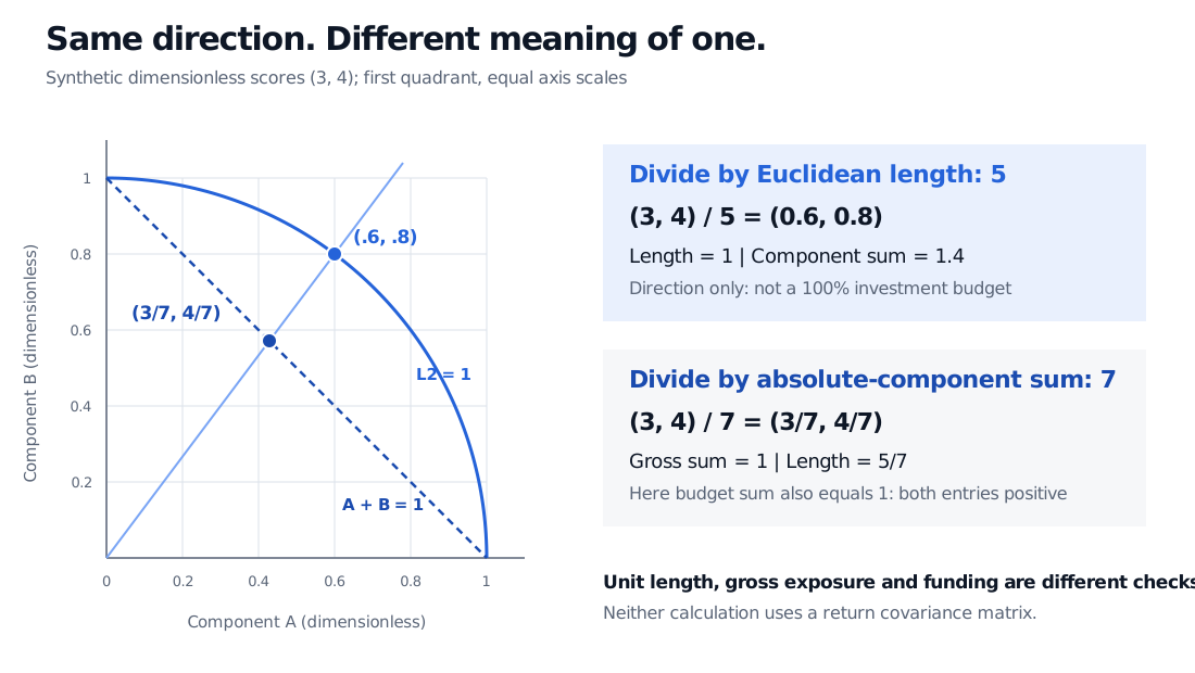
Suppose a research model produces two synthetic dimensionless scores,

\mathbf{x}=(3,4)

. They express a proposed relative allocation of three parts asset A to four parts asset B. They are scores, not yet funded portfolio weights.

The length is $\sqrt{3^2+4^2}=5$ , giving

\mathbf{u}=(0.6,0.8), \qquad 0.6^2+0.8^2=1, \qquad 0.6+0.8=1.4.

If these numbers were used as portfolio weights, they would allocate 60% of net asset value to A and 80% to B. The risky allocations total 140%. Completing the balance sheet with cash would require a cash weight of $1-1.4=-0.4$ : borrowing 40% of net asset value, before costs and restrictions. Unit length has not supplied a fully invested, unlevered allocation.

For this positive score vector, dividing instead by the component sum gives

\mathbf{w}=\frac{(3,4)}{3+4} =\left(\frac37,\frac47\right), \qquad w_A+w_B=1.

Its Euclidean length is $5/7$ , rather than one. Both choices retain the ratio $3:4$ ; they satisfy different targets.

Synthetic dimensionless scores (3,4) give Euclidean unit vector (0.6,0.8), whose component sum is 1.4, and gross-normalised vector (3/7,4/7), whose sum is 1 and Euclidean length is 5/7.

Original synthetic geometry. The first quadrant uses equal axis scales: the same score ray meets the unit circle and the long-only budget line at different points. No return covariance or market data is used.

Gross exposure and net funding part ways with shorts

The Manhattan norm gives another legitimate norm-based rule:

\mathbf{g}=\frac{\mathbf{x}}{\lVert\mathbf{x}\rVert_1}, \qquad \lVert\mathbf{x}\rVert_1=\sum_i\lvert x_i\rvert, \qquad \sum_i\lvert g_i\rvert=1.

When components represent comparable signed asset exposures relative to the same net asset value, this sets gross exposure to 100%. The positive denominator preserves long and short signs. With nonnegative scores, it agrees with dividing by the ordinary sum, as it does for

(3,4)

With shorts, the distinction matters. The nonzero vector $(1,-1)$ has Euclidean length $\sqrt2$ and absolute-component sum $2$ , but ordinary sum zero. Gross normalisation gives $(1/2,-1/2)$ : 100% gross risky exposure, zero net risky exposure. It does not invest the cash balance; cash and funding must be accounted for separately.

By contrast, the budget-sum rule

\mathbf{b}=\frac{\mathbf{x}}{\sum_i x_i}

is undefined for $(1,-1)$ . It can also reverse every sign when the denominator is negative: $(1,-2)$ becomes $(-1,2)$ . When the sum is close to zero, the resulting positions can be very large. An ordinary signed sum is not a norm, so budget scaling has different existence and sign properties.

Unit length does not mean unit risk

For a vector of risky-asset weights $\mathbf{w}$ and a return covariance matrix $\Sigma$ , model portfolio volatility is

\sigma_p=\sqrt{\mathbf{w}^{\mathsf T}\Sigma\mathbf{w}}.

Given a positive volatility target $\sigma_*$ , a positive current $\sigma_p$ and a fixed covariance model, scaling the risky weights to

\widetilde{\mathbf{w}} =\frac{\sigma_*}{\sigma_p}\mathbf{w}

makes their model volatility equal to $\sigma_*$ . The target and covariance must use the same return horizon and annualisation convention. This calculation assumes linear portfolio-return accounting, with any balancing cash treated as risk-free over that horizon. It may require borrowing or leave cash uninvested; budget, leverage and trading constraints still have to be satisfied. Estimated covariance can be wrong, so the formula sets model risk, not guaranteed future realised volatility. If $\sigma_p=0$ , it cannot scale the vector to a positive target.

Euclidean normalisation uses component squares alone. Risk scaling uses the quadratic form defined by covariance, including different asset volatilities and their relationships. The two operations answer different questions.

Finally, choose the coordinate units before choosing a norm. Components measured in a common currency and on a common exposure basis can be scaled together. Combining an amount in USD with a sensitivity in USD per basis point needs explicit component scales or another justified metric first. Dividing the resulting numbers by their length cannot repair an arbitrary unit choice. Component-by-component rescaling changes the geometry; it is a separate decision from scaling the entire vector.

For the algebra behind length and unit vectors, see The Dot Product, Length, and Angle (public preview; full lesson requires membership).

Sources

Boyd, S. and Vandenberghe, L. Introduction to Applied Linear Algebra: Vectors, Matrices, and Least Squares, Cambridge University Press, 2018, §§3.1–3.2, §5.3 and §17.1.1: norms, coordinate units, normalised vectors and portfolio accounting. Authors' book page.
Strang, G. Introduction to Linear Algebra, 5th ed., Wellesley-Cambridge Press, 2016, §1.2, pp. 13–14: unit vectors and division by nonzero length.
Snyder, W. Linear Algebra, Geometry, and Computation, “Analytic Geometry in $\mathbb{R}^n$ ,” subsection “Normalization to Unit Length.” Boston University course text.
Boyd, S. et al. “Multi-Period Trading via Convex Optimization,” Foundations and Trends in Optimization 3(1), 2017, §4.2: covariance-based portfolio risk. Author-hosted paper.

Divide the whole vector by one positive number

A signal direction is not an investment budget

Gross exposure and net funding part ways with shorts

Unit length does not mean unit risk

Sources

Related terms

Euclidean norm

Manhattan norm

Orthogonal vectors

Quadratic form

Vector