Manhattan norm: Definition & Examples

The Manhattan norm, or L1 norm, is the sum of the absolute values of a vector's coordinates. For a real vector

\mathbf{x}=(x_1,\ldots,x_n)

\lVert\mathbf{x}\rVert_1=\sum_{i=1}^n\lvert x_i\rvert.

Signs disappear before addition:

\lVert(3,-4)\rVert_1=3+4=7

, rather than

-1

. The associated Manhattan distance between two vectors is

\lVert\mathbf{x}-\mathbf{y}\rVert_1

. Its name recalls a rectangular street grid: travelling three blocks east and four south takes seven blocks of travel, even though the straight-line distance is five.

In portfolio work, this distinction is cash-relevant. Selling one asset and buying another creates two trading legs. Their signed changes can sum to zero while both incur costs.

A USD 100 transfer creates USD 200 of trading

Consider a hypothetical portfolio with USD 1,000 of pretrade net asset value (NAV). At unchanged execution prices, its two asset weights move from

\mathbf{w}^{\mathrm{old}}=(0.6,0.4) \quad\text{to}\quad \mathbf{w}^{\mathrm{target}}=(0.5,0.5).

Both vectors use the same pretrade NAV denominator. There are no external deposits or withdrawals, and the target is specified before fees. Thus

\Delta\mathbf{w}=(-0.1,0.1)

: sell USD 100 of asset A and buy USD 100 of asset B.

Quantity	Calculation	Result
Signed weight change	$-0.1+0.1$	$0$
L1 distance between allocations	$\lvert-0.1\rvert+\lvert0.1\rvert$	$0.2$
Total dollars traded, both legs	$1{,}000\times0.2$	USD 200
One-way turnover	$\frac12\times0.2$	$0.1$ , or 10%

The half appears because purchases equal sales in this fee-free, no-flow rebalance: each is USD 100. More generally, whenever $\sum_i\Delta w_i=0$ ,

\sum_i\max(\Delta w_i,0) =\sum_i\max(-\Delta w_i,0) =\frac12\lVert\Delta\mathbf{w}\rVert_1.

We call

\lVert\Delta\mathbf{w}\rVert_1

gross, or two-way, turnover, and half of it one-way turnover here. Reports can use different conventions, denominators and asset coverage; check which one a quoted turnover number uses. A change between two historical weight snapshots also includes price-driven drift, so it need not measure executed trading.

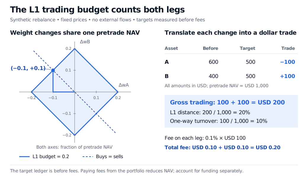
Synthetic rebalance from weights 0.6 and 0.4 to 0.5 and 0.5. Changes minus 0.1 and plus 0.1 lie on an L1 trading-budget diamond of radius 0.2. With USD 1,000 pretrade NAV, sales and purchases are each USD 100, gross trading is USD 200, one-way turnover is 10%, and fees of 0.1% per leg total USD 0.20.

Original synthetic example. Weight changes use a common pretrade NAV, fixed prices and no external flows. The target ledger is before fees; the dashed line enforces equal purchases and sales.

At a hypothetical fee rate of 0.1% on each traded dollar, the fee is

0.001\times(100+100)=\text{USD }0.20.

Multiplying that rate by the one-way USD 100 amount would miss half the fee. For a common symmetric rate

c

and reference NAV

V

, the proportional-cost estimate is

cV\lVert\Delta\mathbf{w}\rVert_1

. Asset-specific buy and sell rates require separate weighted terms; fixed tickets and market impact need a richer model. See MOSEK's transaction-cost formulation for that distinction and the funding constraint.

Fees also consume wealth. If the two USD 100 asset trades are kept fixed and the fee is debited to a cash account, the assets total USD 1,000, cash is USD −0.20, and NAV is USD 999.80 before any financing charge. If a cash debit is disallowed, the trades must be adjusted to fund the fee. The pre-fee 50/50 target cannot silently be treated as exact final weights relative to an unchanged USD 1,000 NAV.

The geometry of an absolute-change budget

In two dimensions,

\lvert x_1\rvert+\lvert x_2\rvert\le1

describes a filled diamond, with vertices

(1,0)

(0,1)

(-1,0)

and

(0,-1)

. This is the L1 unit ball. A trading constraint

\lVert\Delta\mathbf{w}\rVert_1\le b

scales that diamond to radius $b$ . In the figure, $b=0.2$ ; intersecting it with the equal-buy-and-sell line $\Delta w_A+\Delta w_B=0$ leaves a feasible line segment. The selected trade sits at one endpoint. A 20% gross trading budget therefore allows at most 10% one-way turnover under these assumptions.

The budget is convex and can be expressed without an absolute-value operator by introducing auxiliary variables:

-u_i\le\Delta w_i\le u_i,\qquad u_i\ge0,\qquad \sum_i u_i\le b.

Feasibility is equivalent to the original budget: any feasible $u_i$ must be at least $\lvert\Delta w_i\rvert$ , and choosing equality works whenever the budget holds. This is why absolute trading costs fit naturally into convex portfolio optimisation, despite their kink at zero.

Choose the norm for the economic question

For comparable coordinates, L1 is zero only at the zero vector, scales as $\lVert a\mathbf{x}\rVert_1=\lvert a\rvert\lVert\mathbf{x}\rVert_1$ , and obeys the triangle inequality. The last property follows by summing $\lvert x_i+y_i\rvert\le\lvert x_i\rvert+\lvert y_i\rvert$ coordinate by coordinate.

Compare three legitimate summaries of $(3,-4)$ :

Norm	Value	Emphasis
Manhattan, L1	$7$	Sum of all absolute components
Euclidean, L2	$5$	Root-sum-square length
Maximum, L-infinity	$4$	Largest absolute component

For $n\ge1$ , they satisfy

\lVert\mathbf{x}\rVert_\infty \le\lVert\mathbf{x}\rVert_2 \le\lVert\mathbf{x}\rVert_1 \le\sqrt{n}\,\lVert\mathbf{x}\rVert_2.

These bounds relate the measures; they do not give them the same financial meaning. Applying L1 to holdings gives absolute exposure; applying it to trades gives total absolute changes. For example, the risky sleeve

(0.6,-0.8)

has gross exposure of

1.4

, or 140% of NAV, but L2 norm

1

and maximum norm

0.8

. This is a sleeve, not a fully invested two-asset budget. None of these numbers alone is portfolio volatility, which also needs asset covariances.

Units and coordinate choices matter. Adding raw dollar prices to yield changes in basis points does not produce a coherent financial distance. Explicit positive component scales

s_i

give dimensionless coordinates

z_i=x_i/s_i

and distance

\sum_i\lvert x_i-y_i\rvert/s_i

. Apply the same scales to both vectors. The chosen scales specify how much each difference counts; they are part of the model. L1 also depends on the chosen axes, so changing from asset exposures to rotated factor coordinates generally changes the norm.

For the portfolio applications, Turnover and the Information Horizon develops drift and the one-way convention. Transaction Costs and Implementation develops proportional costs and the no-trade zone created by their kink. Both offer public previews; full lessons require membership.

Sources

Stephen Boyd and Lieven Vandenberghe, Introduction to Applied Linear Algebra: Vectors, Matrices, and Least Squares, Exercise 3.5 and §17.1.1: L1 and maximum norms, and absolute portfolio weights.
David Bindel, Cornell CS 6210, “Introduction”, 25 August 2025, “Properties of a norm”, “Concrete space norms” and “Norm equivalence”.
MOSEK, Portfolio Optimization Cookbook, Chapter 6, “Transaction costs”, especially §6.1: proportional buy/sell costs and the self-financing budget.
Stanford Convex Optimization Group, “Portfolio optimization”, “Portfolio constraints” and “Variations”: absolute-weight leverage limits and transaction-cost penalties.

A USD 100 transfer creates USD 200 of trading

The geometry of an absolute-change budget

Choose the norm for the economic question

Sources

Related terms

Absolute value

Euclidean norm

Maximum norm

Vector

Volatility